9th International Conference PROCESS CONTROL 2010 June 7 – 10, 2010, Kouty nad Desnou, Czech Republic _____________________________________________________________________________________________________
INVERTED PENDULA SIMULATION AND MODELING A GENERALIZED APPROACH JADLOVSKÁ SLÁVKA, JADLOVSKÁ ANNA Department of Cybernetics and Artificial Intelligence, Faculty of Electrical Engineering and Informatics, Technical University of Košice, Letná 9, 04201 Košice, Slovak Republic, e-mail:
[email protected],
[email protected] Abstract: The aim of this paper is to provide a complex view of the modeling and simulation of inverted pendula systems. Crucial modeling procedures such as the derivation of differential motion equations for inverted pendula systems and symbolic linearization with respect to a given equilibrium point are presented in form of symbolic MATLAB algorithms, generalized for a system of n inverted pendula. The algorithms are then used to derive accurate mathematical models of a single and double inverted pendulum as well as their linear approximations. The paper then presents Inverted Pendula Modeling and Control, a thematic Simulink block library designed by the authors. As part of the library, the open-loop dynamics of the models is analyzed in a series of simulation experiments and a set of suitable state-space control algorithms that stabilize the pendulum in the inverted position is designed and supported by a set of library blocks. Keywords: nonlinear dynamical system, system of inverted pendula, generalized modeling, statespace control, MATLAB/Simulink block library
1 INTRODUCTION Inverted pendula systems represent a significant group of mechanical systems used in control education with a variety of practical applications, including (see [Jadlovská, 2009], [Sultan, 2004]): • simulation of the unstable system of a human or robotic upper limb if the center of pressure is placed below its center of gravity • modeling a human or a robot standing upright • simulation of a space shuttle or a rocket taking off • missile guidance, if thrust is actuated at the bottom of a tall vehicle Thorough physical analysis is generally required to obtain mathematical expressions that model the real system dynamics with such accuracy that it is possible to use them as substitutes in case a laboratory model is unavailable. Despite the fact that inverted pendula analytical identification is considered a well-explored matter and the equations of motion of this type of a system are standardly included in a number of sources (e.g. [Schlegel et al., 2005] provides the equations for a single, double and triple pendulum model), a general algorithm, which would output the equations of motion for any given number of pendula, has not yet been introduced. Since the force summation method based on Newton’s laws of motion tends to be error-prone and cannot be easily transformed into an algorithm, this paper uses the Lagrange approach to perform the derivation of the motion equations. In order to obtain as precise an approximation of the real model dynamics as possible, Rayleigh dissipation function that describes the viscous system damping and friction was integrated in the standard Euler-Lagrange equation. The biggest advantage of the Lagrange mechanics employment is that it can be easily algorithmized into a MATLAB function (m-file). In a similar generalized way, a linearized model, which is necessary for any linear feedback controller design, is created. The use of linear controllers upon nonlinear systems is justified by the easily verifiable assumption that the behavior of a linear approximation near to the equilibrium point shows little error compared to the nonlinear original. Block libraries represent the object-oriented, event-flow-driven, user-friendly problem-solving approach within the MATLAB/Simulink environment. Through the Simulink Library Browser, a number of pre-installed (Toolbox) libraries can be accessed and used to solve or simulate various scientific and technical issues by means of block interconnecting. Furthermore, to provide a wider variety of problems with such user flexibility, custom masked blocks may be created and grouped into
C134a – 1
9th International Conference PROCESS CONTROL 2010 June 7 – 10, 2010, Kouty nad Desnou, Czech Republic _____________________________________________________________________________________________________
user-designed libraries. The final section of the paper describes a block library which was developed to provide such software support for the simulation and control of inverted pendula systems. 2 MATHEMATICAL MODELING 2.1 Motion Equations Derivation – General Procedure The nonlinear mechanical SIMO system of n inverted pendula on a cart is composed of n homogenous, isotropic rods which are joint-bound together and attached to a stable moving base. The input of such a system is the force acting upon the cart; the multiple, i.e. n + 1 outputs are represented by cart position [m] and pendula angles [rad ] . Only the cart position is directly affected by the input force, therefore any system of inverted pendula is considered to be under-actuated. This section outlines the theoretical background, assumptions and derived formulas that led to the creation of an algorithm which derives the equations of motion for any given number of pendula attached to a cart. The algorithm was implemented into MATLAB under the name of invpenderiv.m. The number of pendula needs to be specified as the function parameter. Throughout the derivation process, we assume that • all motion is bound to the xy plane with the cart moving along the line identical to x axis, which at the same time represents the projection of the zero potential energy level into the xy plane • the value of every angle is determined clockwise from the upright position • all parameters are indexed in the following manner: 0 is assigned to the cart, 1 to n represent the individual pendula starting with the pendulum rod attached directly to the cart Let us first introduce a vector of generalized coordinates, which correspond to the system’s n + 1 degrees of freedom, i.e. its outputs: θ(t ) = (θ 0 (t ) θ 1 (t ) K θ n (t ) ) (1) The Euler-Lagrange equations represent the system’s degrees of freedom each and in the condensed vector form they appear as: T
d ∂L(t ) ∂L(t ) ∂D (t ) − + = Q * (t ) (2) dt ∂θ& (t ) ∂θ(t ) ∂θ& (t ) where Lagrange function (Lagrangian) is defined as the difference between the system’s kinetic and potential energy L(t ) = E K θ(t ), θ& (t ) − E P (θ(t )) (3) Rayleigh (dissipative) function describes the viscous (friction) forces within the system D(t ) = D θ& (t ) (4)
(
)
( )
and Q (t ) is the vector of generalized external forces acting upon the system. From now on, we will use s xi (t ) , s yi (t ) to denote the coordinates of position and vxi (t ) , v yi (t ) *
will denote the velocities in the direction of the axes. The nomenclature of the numerical parameters that describe the system will obey the standard conventions: mi [kg ] – mass of the cart ( i = 0 ) and the pendula ( i = 1 to i = n ) l i [m] – length of i -th pendulum
[ ] δ [kgs ] , [kgm s ] g ms −2
−1
–
gravitational acceleration ( g = 9,81ms −2 will be used)
2 −1
– friction coefficient of the cart against the surface ( i = 0 ) / damping constant related to the pivot point of i -th pendulum (i = 1to i = n) i
Construction of Lagrange motion equations: Out of all considered subsystems, only the dynamics of the cart is directly affected by the external force acting upon the system. Therefore, the vector of external forces has the following form: Q * (t ) = (F (t ) 0 K 0 )
T
(5)
C134a – 2
9th International Conference PROCESS CONTROL 2010 June 7 – 10, 2010, Kouty nad Desnou, Czech Republic _____________________________________________________________________________________________________
Since the total energy of a multi-body system is given as the sum of energies that befit the individual bodies, the relations that characterize a system of n inverted pendula on a cart are: n
EK (t ) =
n
∑ E (t ) ,
n
Ki
E P (t ) =
i =0
n
n
∑ E (t ) , D(t ) = ∑ D (t ) Pi
(6)
i
i =0
i =0
The use of Lagrange equations therefore transforms the process of deriving the motion equations into the determination of kinetic, potential and dissipation energies for the cart and all pendula. These need to be expressed in terms of the generalized coordinates.
Energetic balance of the cart: Assuming the cart’s motion to be linear, we can describe it mathematically using a single spatial dimension. Identifying it as the x axis, the only position coordinate is denoted as s x 0 (t ) = θ 0 (t ) . Therefore, the potential energy of the cart equals E P 0 (t ) = 0 (see assumptions in 2.1). The kinetic energy and the dissipation function both depend on the cart’s velocity: EK 0 (t ) =
1 1 m0vx20 (t ) = m0θ&02 (t ) 2 2 1 1 D0 (t ) = δ 0 v x20 (t ) = δ 0θ&02 (t ) 2 2
(7) (8)
Energetic balance of i-th pendulum: Let us suppose that the whole mass of a pendulum rod is concentrated in its center of gravity (CoG) which is identical to the geometrical center of the rod in the distance of l i from the pivot point. 2
The coordinates of the CoG of i-th pendulum rod are hence expressed as: i l θ 0 (t ) + lk sin θ k (t ) − i sin θi (t ) s ( t ) xi 2 k =1 i s yi (t ) = li ( ) ( ) l cos θ t − cos θ t k k k 2 k =1 while the velocities in the direction of the axes equal:
∑
∑
n & l θ 0 (t ) + lkθ&k (t )cosθ k (t ) − i θ&i (t )cosθi (t ) vxi (t ) 2 k =1 i v yi (t ) = l − l θ& (t )sin θ (t ) + i θ& (t )sin θ (t ) k k k i i 2 k =1 The potential energy of i -th pendulum is defined by the height of the CoG above the x axis:
(9)
∑
∑
(10)
i l (11) EPi (t ) = mi gs yi (t ) = mi g lk cos θ k (t ) − i cos θ k (t ) 2 k =1 and the kinetic energy of each pendulum is a sum of two expressions that describe the pendulum’s translational and rotary motion:
∑
EKi (t ) = where J Ti =
1 1 mi vi2 (t ) + J Tiθ&i2 (t ) 2 2
(12)
1 mi l i2 is the pendulum’s moment of inertia with respect to the center of gravity and 12
v i (t ) = v xi2 (t ) + v 2yi (t ) is the magnitude of i -th pendulum translational velocity.
The dissipation properties of the i -th pendulum depend quadratically on the angular velocities of pendulums marked as i and i − 1 :
C134a – 3
9th International Conference PROCESS CONTROL 2010 June 7 – 10, 2010, Kouty nad Desnou, Czech Republic _____________________________________________________________________________________________________
(
Di (t ) =
)
2 1 δ i θ&i (t ) − θ&i −1 (t ) (13) 2 1 which yields Di (t ) = δ i θ&i2 (t ) if n = 1 . 2 The functions of MATLAB’s Symbolic Math Toolbox enabled us to include the abovementioned physical relationships in the invpenderiv.m and, furthermore, to generate a simplified and rearranged form of the equations, equivalent to the most likely form obtained by manual derivation. An example of the command window output produced by invpenderiv.m is listed in [Jadlovská et al., 2009]. In addition to the eventual symbolic motion equations in the “pretty” form, all physically significant steps of the derivation process are displayed and can be tracked.
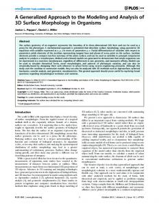
Fig. 1 – Single and double inverted pendulum on a cart – scheme and basic nomenclature
2.2 Single and Double Inverted Pendulum By setting n to 1, we obtain a system of a single inverted pendulum (Fig. 1, left), which is composed of a pendulum rod attached to the cart. The eq=invpenderiv(1) command was used to obtain the model which consists of second-order nonlinear differential equations that describe the cart subsystem: (m0 + m1 )θ&&0 (t ) + δ 0θ&0 (t ) + 1 m1l1 θ&&1 (t )cosθ1 (t ) − θ&12 (t )sin θ1 (t ) = F (t ) (14) 2 and the pendulum subsystem: 1 1 J1θ&&1 (t ) + δ1θ&1 (t ) + m1l1θ&&0 cosθ1 (t ) − m1 gl1 sin θ1 (t ) = 0 (15) 2 2 1 where J 1 = m1 l12 stands for the pendulum’s moment of inertia with respect to the pivot. 3 Connecting a couple of rigid rods in a joint and attaching one of these to a cart produces a system of a double inverted pendulum (Fig. 1, right). Analogically to the single inverted pendulum system, eq=invpenderiv(2) returns the second-order nonlinear differential equations that describe the cart subsystem: (m0 + m1 + m2 )θ&&0 (t ) + δ 0θ&0 (t ) + 1 m1l1 + m2l1 θ&&1 (t )cosθ1 (t ) − θ&12 (t )sin θ1 (t ) + 2 (16) 1 2 + m2l2 θ&&2 (t )cosθ 2 (t ) − θ&2 (t )sin θ 2 (t ) = F (t ) 2 the lower pendulum subsystem: 1 J1 + m2l12 θ&&1 (t ) + (δ1 + δ 2 )θ&1 (t ) − δ 2θ&2 (t ) + m1l1 + m2l1 θ&&0 (t )cosθ1 (t ) + 2 (17) 1 1 2 & & & m2l1l2 θ2 (t )cos(θ1 (t ) − θ 2 (t )) + θ2 (t )sin(θ1 (t ) − θ2 (t )) − m1 + m2 gl1 sinθ1 (t ) = 0 2 2
(
)
(
(
(
)
)
)
(
)
C134a – 4
9th International Conference PROCESS CONTROL 2010 June 7 – 10, 2010, Kouty nad Desnou, Czech Republic _____________________________________________________________________________________________________
and the upper pendulum subsystem: 1 J 2θ&&2 (t ) + δ 2 θ&2 (t ) − θ&1 (t ) + m2l2θ&&0 (t )cosθ 2 (t ) + 2 (18) 1 1 2 + m2l1l2 θ&&1 (t )cos(θ1 (t ) − θ 2 (t )) − θ&1 (t )sin (θ1 (t ) − θ 2 (t )) − m2 gl2 sin θ 2 (t ) = 0 2 2 1 1 2 2 where J 1 = m1l1 , J 2 = m 2 l 2 stand for the moments of inertia of the lower and upper pendulum 3 3 with respect to their pivot points. The automatically generated nonlinear differential equations were, in both cases, identical to the equations derived manually (compare (15),(16) to [Roubal, 2002], [Schlegel et al., 2005], (17)-(19) to [Bogdanov, 2004], [Demirci, 2004]), which confirms the validity of the algorithm. It is worth noting that the complete derivation procedure in the case of a double and triple inverted pendulum, as it was included e.g. in [Schlegel et al., 2005], need not have been done. The general physical relationships listed in 2.1 instead imply that once the single inverted pendulum model has been derived, all energetic balances related to the cart and the lower pendulum of a double inverted pendulum system are already known and only those which describe the upper pendulum need to be computed.
(
)
(
)
3 LINEAR APPROXIMATION OF INVERTED PENDULA SYSTEMS We will next focus on the analysis of inverted pendula systems based on the state-space theory of continuous dynamical systems, which describes a nonlinear SIMO system with use of a differential state equation and an algebraic output equation: x& (t ) = f (x(t ), u (t ), t ) , (19) y (t ) = g(x(t ), u (t ), t ) where x(t ) is the state vector, u (t ) is the scalar input value, y (t ) is the output vector. Among the conclusions drawn from the analysis above was that the order of a system of n inverted pendula on a cart is 2n + 2 . Therefore, a state vector in the following form was introduced to describe the system:
(
)
T T x(t ) = θ(t ) θ& (t ) = (x1 (t ) x 2 (t ) ... x 2 n + 2 (t )) and the force acting upon the cart was logically defined as the only input of the system:
(20)
u (t ) = F (t ) (21) The output equation is defined in such a way so that vector y (t ) would either represent the vector of generalized coordinates θ(t ) , or the whole state vector (19), if necessary. To determine the state
(
)
T equation x& (t ) = θ& (t ) &θ&(t ) , the Lagrange motion equations need above all to be rewritten into the socalled minimal ODE form M (θ(t ))&θ&(t ) + N θ(t ), θ& (t ) θ& (t ) + P (θ(t )) = V (t ) (22)
(
)
which makes it possible to isolate the derivative of state-space vector: θ& (t ) θ& (t ) = (23) &θ&(t ) (M(θ(t )))−1 V(t ) − N θ(t ), θ& (t ) θ& (t ) + P θ& (t ) in which every element of θ(t ) , θ& (t ) can be substituted by its x(t ) counterpart. The fact that a nonlinear autonomous dynamic system has no tendency to change its state if in equilibrium corresponds to equalities x& (t ) = 0 and u (t ) = u S = 0 (24) By solving these, we obtain the p equilibrium points of the system ( j = 1,2,..., p ):
(
j xS
= (x1S
x2 S
(
)
( ))
... x(2 n + 2 )S )
T
(25)
C134a – 5
9th International Conference PROCESS CONTROL 2010 June 7 – 10, 2010, Kouty nad Desnou, Czech Republic _____________________________________________________________________________________________________
With use of the Taylor series, we can now create the linear approximation to the whole state equation by substituting f i (x(t ), u (t )) by f i* (x(t ), u (t )) : f i* (x(t ), u (t )) ≈ f i (x S , uS ) +
2n+ 2
∑ k =1
∂f i (x(t ), u (t )) ∂xk (t ) x
S ,u S
(xk (t ) − xkS ) + ∂fi (x(t ), u (t )) ∂u (t ) x
(u (t ) − uS ) S
(26)
,u S
For the case of the upright position, the equilibrium is x (t ) = x S = 0 T and since u (t ) = uS = 0 , and the state-space description of the physically realizable linearized system is given as x& (t ) = Ax(t ) + bu (t ) (27) y (t ) = Cx(t ) The described transformation of the Lagrange mathematical model into a state-space matrix form was implemented into MATLAB. Since the complexity of symbolic matrices increases greatly with increasing order of the system, only the state-space matrices of the single inverted pendulum model in the upright position, produced by matrices_single.m, are displayed here as an example. 0 0 1 A = 0 0
0
1
0 − 3m1 g 4 m0 + m1 6 g (m0 + m1 ) l1 (4 m0 + m1 )
0 − 4δ 0 4 m0 + m1 6δ 0 l1 (4 m0 + m1 )
0 1 0 6δ 1 4 1 0 0 0 1 1 b = 4m + m C = 0 1 0 0 l1 (4 m0 + m1 ) 0 1 − 12δ 1 (m0 + m1 ) 6 − l (4 m + m ) m1l12 (4 m0 + m1 ) 0 1 1 0
(28)
Once again, the command window output of the function can be previewed in [Jadlovská et al., 2009]. The generated state-space matrices were proved to be accurate (compare (28) to [Schlegel, 2005]).
4 IPMAC – INVERTED PENDULA MODELING AND CONTROL (SIMULINK BLOCK LIBRARY) A structured Simulink block library under the name of Inverted Pendula Modeling and Control (IPMaC) was designed to provide software support for the analysis and synthesis of inverted pendula systems. The IPMaC can be fully integrated into the Simulink Library Browser and used identically to the pre-installed Simulink block libraries. The following section provides a brief insight into the library’s functionality.
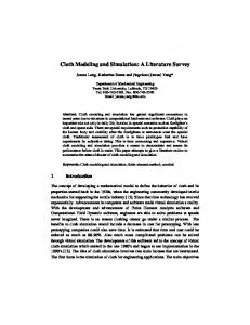
Fig. 2 – Simulink blocks of inverted pendula models included in the IPMaC library
4.1 Open-Loop Dynamical Analysis The mathematical models of a single and double inverted pendulum were implemented into the programming environment of MATLAB/Simulink in form of atomic library blocks: Single Inverted Pendulum on a Cart and Double Inverted Pendulum on a Cart; both with their own icon and a dynamical parametric block mask. The block mask of each implemented system makes it possible to C134a – 6
9th International Conference PROCESS CONTROL 2010 June 7 – 10, 2010, Kouty nad Desnou, Czech Republic _____________________________________________________________________________________________________
change the system’s parameters, specify the initial conditions (which enable the initial deflection analysis), enable or disable the input force and adjust the number of outputs, which is equivalent to equipping a real model with sensors. The blocks themselves have a cell structure, i.e. each nonlinear equation that is part of the system’s mathematical model corresponds to a subsystem block interconnected with the others with respect to their mutual physical relations. As an illustration, Fig. 3 and Fig. 4 depict the inner structure of subsystem blocks Cart and Pendulum within the Single Inverted Pendulum on a Cart block, both of which represent an exact transformation of nonlinear equations into Simulink block diagrams. 1 F
3 4 dfi 1/dt d2fi /dt2
2 fi 1
s ds/dt d2s/dt2
cossin
clen
-K-
d2fi 0dt
-K-
(m1*l1)/2
1 xo s
d2fi 0dt
1/(m0+m1)
-C-
dfi 0dt
-C-
Integrator
init (3)
1 xo s
dfi 0dt
1 fi 0
fi 0
Integrator 1
init (1)
-K-
2 dfi 0/dt
delta 0
3 d2fi 0/dt2
Fig. 3 – The Cart subsystem within the function block Single Inverted Pendulum on a Cart 1 d2fi 0/dt 2
-Kcos cosine function
Dot Product sin sine function
(m 1*l1)/2
-K(m1*g*l1)/2
-K1/J1
d2fi 1dt d2fi 1dt
-C-
xo
1 s
init (4) Integrator 2 -K-
dfi 1dt dfi 1dt
-Cinit (2)
xo
1 s
fi 1 fi 1
1 fi 1
Integrator 1
delta 1 2 dfi 1/dt 3 d2fi 1/dt 2
Fig. 4 – The Pendulum subsystem within the function block Single Inverted Pendulum on a Cart
Creating complete and functional simulation models of inverted pendula on a cart in form of an atomic icon allows for detailed observation of their dynamics with no additional modeling apart from input/output block affiliation. The analyses of the open-loop dynamical behavior of both the single and double inverted pendulum system were performed as a response to a signal constrained in terms of time and amplitude, included in the IPMaC as the Impulse block. To view the signals generated during simulation, Scope and Scope rad2deg blocks were used, the latter displaying the signal in degrees rather than in radians. Both schemes can be run from the Demo Simulations section of the IPMaC, which is basically a collection of links to simulation schemes whose purpose is to solve various analysis- and synthesis-related problems. The schemes are composed nearly exclusively of the IPMaC blocks. The dynamics of single inverted pendulum system was analyzed for two groups of parameters: group I: m 0 = 0.3kg , m1 = 0.275kg , l1 = 0.5m , δ 0 = 0.3kgs −1 , δ 1 = 0.01148kgm 2 s −1 group II: m 0 = 0.1kg , m1 = 1kg , l1 = 0.8m , δ 0 = 0.3kgs −1 , δ 1 = 0.1kgm 2 s −1 and the numeric values used in the double inverted pendulum system simulation were: m 0 = 0.3kg , m1 = 0.275kg , m 2 = 0.275kg , l1 = 0.5m , l 2 = 0.5m , δ 0 = 0.3kgs −1 , δ 1 = 0.1kgm 2 s −1 ,
δ 2 = 0.1kgm 2 s −1 If we take a closer look at the simulation results (Fig. 5, Fig. 6), several conclusions can be drawn independently of the number of pendula attached to a cart: From the moment the cart starts to move as a response to the time-constrained input force impulse, its velocity decreases through time and gradually comes down to zero because of the present friction. All pendula fall in counterdirection to the cart (1st Newton Law of inertia), passing through
C134a – 7
9th International Conference PROCESS CONTROL 2010 June 7 – 10, 2010, Kouty nad Desnou, Czech Republic _____________________________________________________________________________________________________
oscillatory transient state before finally stabilizing themselves in the stable equilibrium point in which they are all pointing downward. The backward impact of each pendulum on the cart, which increases with the weight of the load attached, is also visible. Since such open-loop behavior is correct compared to generally known empirical observations of pendula behavior, it can be concluded that both models display acceptable overall performance. Cart Position Analysis - Single Inverted Pendulum
Pole Angle Analysis - Single Inverted Pendulum
1.4
0
Pole Angle - ParamGroup1 Pole Angle - ParamGroup2
1.2 Cart Position - ParamGroup1 Cart Position - ParamGroup2
-50
1
Pole Angle [deg]
Cart Position [m]
-100 0.8
0.6
0.4
-150
-200 0.2
-250 0
-0.2 0
2
4
6
8
10
12
14
16
18
-300 0
20
2
4
6
8
Simulation time [s]
10
12
14
16
18
20
Simulation time [s]
Fig. 5 – Single Inverted Pendulum on a Cart - cart position and pendulum angle Pole Angle (Lower & Upper) Analysis - Double Inverted Pendulum
Cart Position Analysis - Double Inverted Pendulum
50
1.4
0 Pole Angle (Lower) Pole Angle (Upper)
Cart Position
1.2
-50
Pole Angle [deg]
Cart Position [m]
1
0.8
0.6
0.4
-150
-200
-250
-300
0.2
0 0
-100
-350 0 2
4
6
8
10
12
14
16
18
2
4
6
8
10
12
14
16
18
20
Simulation time [s]
20
Simulation time [s]
Fig. 6 – Double Inverted Pendulum on a Cart – cart position, upper and lower pendula angles
4.2 Verification of State-Space Control Algorithms The continuous linear feedback methods were employed to demonstrate the controllability properties of the simulation model of single inverted pendulum. The control objective was to stabilize the pendulum in the upright (inverted) i.e. unstable position, i.e. to maintain the equality 1 x (t ) = 0 T , while the individual approached problems were: • initial deflection of the pendulum (nonzero initial conditions) • compensation of a time-constrained disturbance input signal • tracking a required position of the cart or a combination of the three. The pendulum had to be kept upright in any case. It is known (e.g. from [Jadlovská, 2009], [Demirci, 2004], [Jadlovská, 2003]) that if a feedback gain k is applied on a measurable full state vector x(t ) , it brings the system to the origin of the state space. A specified nonzero required value w(t ) requires an additional, setpoint gain k v . The control law was therefore constructed in form of the following sum: u (t ) = u f (t ) + u v (t ) + d u (t ) = −kx(t ) + k v w(t ) + d u (t )
(29)
where u f (t ) = −kx(t ) is the feedback component, uv (t ) = k v w(t ) is the setpoint component and d u (t ) is the unmeasured disturbance input. As such, the control law is evaluated within the State Space Controller (SSC) block from the IPMaC. The block’s dynamic mask allows the user to pick the method to determine the feedback gain vector k : the pole-placement algorithm or the linear quadratic regulation (LQR) optimal control method are available, both of which are supported by Control Toolbox in form of built-in functions (acker/place, lqr). The nonzero setpoint input w(t ) and disturbance input d u (t ) may optionally be enabled or disabled so as to adjust the block’s appearance to match the control objective. C134a – 8
9th International Conference PROCESS CONTROL 2010 June 7 – 10, 2010, Kouty nad Desnou, Czech Republic _____________________________________________________________________________________________________
In case we suppose that measurement limitations make it impossible to retrieve the state space vector as a whole, an estimator is included in the control loop to provide the approximated (reconstructed) state vector xˆ (t ) . The principle of Luenberger state estimator lies in the gradual minimization of the estimation error ~ x (t ) = x(t ) − xˆ (t ) . To keep the time behavior of the error independent of system parameters, i.e. to maintain: ~ x& (t ) = (A − LC )~ x (t ) (30) where L is the estimator gain matrix, the estimator creates a model of the original system in the form: x&ˆ (t ) = A xˆ (t ) + b u (t ) + L (y (t ) − C xˆ (t )) (31) which is the relation evaluated within the State Estimator block. Once again, the block mask allows the gain to be determined alternatively through pole-placement or linear quadratic control method, according to the user’s choice. u xe
xe'=Axe+Bu +L(y-ye) y State Estimator
x du
State Space Controller
w
Impulse
Scope
x' = Ax+Bu y = Cx+Du
u
State -Space State Space Controller
Step
Scope rad 2deg
u xe
xe'=Axe+Bu +L(y-ye) y State Estimator 1 0 Constant
fi 0 cart position Scope 1 x
State Space Controller Signal 1
uu
F external force on the cart
w
State Space Controller 1
Signal Builder 1
Scope rad 2deg 1
fi 1 pole angle
Single Inverted Pendulum on a Cart
Fig. 7 – Examples of control simulation schemes
The example schemes above illustrate two ways of interconnecting the blocks that result in a control scheme for the single inverted pendulum system. A simulation scheme of a linearized and a nonlinear model is shown, with the State Space Controller and State Estimator blocks as part of both schemes. The adjustment of the number of block inputs is also demonstrated. As was the case with open-loop analysis, these schemes can be located in the Demo Simulations section of the IPMaC. Fig. 8 and Fig. 9 document the time-dependent behavior for both the cart position and the pendulum angle of the nonlinear single inverted pendulum system in case the control objective is to maintain the desired cart position while keeping the pendulum upright; no disturbance input was considered. In order to use the linear methods of synthesis, the linearization of the nonlinear inverted pendulum system was performed by calling the matrices_single.m function. Using the parameters from group I (section 4.1), the following linear state-space matrices were obtained: 0 0 1 A = 0 0
0 0
1 0
− 3 . 5575 40 . 1024
− 0 . 5275 1 . 5824
0 0 1 , b = 0 . 0604 1 . 7582 − 5 . 2747 − 0 . 6813 0 1
C134a – 9
1 1 , C = 0
0
0
1
0
0 0
(32)
9th International Conference PROCESS CONTROL 2010 June 7 – 10, 2010, Kouty nad Desnou, Czech Republic _____________________________________________________________________________________________________
In Fig. 8, the effect of selecting (−5 − 2 −1.2 + 4i −1.2 − 4i) for the designed poles of the system is shown. The feedback gain vector k of (− 3.3704 17.5934 − 3.1803 − 2.6130) was computed and applied on the system. Fig. 9 depicts the results of a LQR-based controller design. In the ∞
minimized quadratic functional J LQ (t ) = x(t ) Qx(t ) + u f (t )Ru f (t )dt , both weighting matrices are
∫
T
0
diagonal and chosen to be Q = diag (500 0 20 0 ) , R = 1 . The principle of separability allows the feedback and estimator gains to be determined independently of each other, i.e. using a different method. Setting the estimation error matrix poles to (− 40 − 41 − 42 − 43) , which made them about 10 times faster than the controller poles, resulted in the following estimator gain matrix: T
82.5 2.6 1677.5 171.9 . L = 1.0 82.3 40.6 1707.8 Pole Angle Stabilization - Pole Placement
Cart Position - Reference Trajectory (Pole Placement) 4
0.3
Pole Angle Setpoint [deg] Pole Angle [deg]
0.25
3
0.2
2
Pole Angle [deg]
Cart Position [m]
Cart Position Setpoint [m] Cart Position [m]
0.15
0.1
1
0
0.05
-1
0
-2
0
2
4
6
8
10
12
14
16
18
-3 0
20
2
4
6
8
10
12
14
16
18
20
Simulation time [s]
Simulation time [s]
Fig. 8 – Single Inverted Pendulum on a Cart – simulation results for pole-placement control without estimator (cart position, pendulum angle) Cart Position - Reference Trajectory (LQR + Pole-Placement)
Pole Angle Stabilization - LQR + Pole Placement
0.3
5 Cart Position Setpoint [m] Cart Position [m]
Pole Angle Setpoint [deg] Pole Angle [deg]
4
0.25 3
2
Pole Angle [deg]
Cart Position [m]
0.2
0.15
0.1
1
0
-1
-2
0.05
-3 0 -4
-0.05 0
1
2
3
4
5
6
7
8
9
10
-5 0
Simulation time [s]
1
2
3
4
5
6
7
8
9
10
Simulation time [s]
Fig. 9 – Single Inverted Pendulum on a Cart – simulation results for LQR control with pole-placementdesigned estimator (cart position tracking, pendulum angle stabilization)
The simulation results reveal that both control blocks do reasonably well. The ability of the designed blocks to control the system with respect to all above-presented requirements has been demonstrated for both methods, although LQR control produces slightly better results despite the need for an estimator. Overally, the simulation results justify the use of linear control methods to control nonlinear systems.
CONCLUSION The purpose of this paper was to propose an original conception of solving the task of modeling and control of inverted pendula dynamical systems. It focused on demonstrating the analogy which is found when we derive mathematical models for systems of n inverted pendula on a cart for a changing n . Practical importance of symbolic mathematical software was pointed out as Symbolic Math Toolbox was used in the process of development of general symbolic procedures that either yield the equations of motion of inverted pendula systems and hence automatize the mathematical modeling,
C134a – 10
9th International Conference PROCESS CONTROL 2010 June 7 – 10, 2010, Kouty nad Desnou, Czech Republic _____________________________________________________________________________________________________
or perform the symbolic linear transformation of a specified nonlinear system. Such approach should eliminate all factual or numeric errors that should arise during the process of mathematical modeling. The transformation of the derived equations of single and double inverted pendulum system into Simulink block schemes was the basis of the creation of inverted pendula simulation models which were integrated in the IPMaC, a structured Simulink block library designed by the authors of this paper. The core of the library is therefore represented by the dynamic-masked simulation models, pre-prepared for use in open-loop analysis as well as state-space controller design. The IPMaC block library was introduced in [Jadlovská, 2009] and is going through constant improvement process. Using the automatic mathematical model derivation, further expansion of the modeling section should be straightforward. A section on rotary inverted pendula, where the base is moving in a plane rather than in a single coordinate, is being designed to serve as software support for a newly-purchased laboratory model of single rotary inverted pendulum. To enable further verification of the controllability properties of inverted pendula systems, all included systems should also become control plants. Finally, as it was hinted in [Jadlovská et al., 2009], the release of the next version of the IPMaC should contain a notably expanded control section, i.e. a wider variety of controller blocks and control schemes in addition to the already included feedback control algorithms. In summary, we believe that the idea of creating a thematic Simulink library, which would group accurate simulation models of mechanical systems together with useful input/output blocks, suitable controller blocks and demonstration simulations, could find its use for a number of types of dynamical systems. Libraries of hydraulic or electrical systems could follow the steps of the IPMaC, which we consider as a contribution to modeling and control education at technical universities. ACKNOWLEDGEMENTS This research was supported by the Scientific Grant Agency of Slovak Republic under the Vega project Multiagent Network Control Systems with Automatic Reconfiguration (No.1/0617/08), as well as by the Agency for the EU Structural Funds of the Ministry of Education of Slovak Republic under the project: Centre of Information and Communication Technologies for Knowledge Systems (project number: 26220120020). REFERENCES JADLOVSKÁ, S. 2009. Inverted Pendula Modeling and Control [in Slovak]. Bachelor thesis. Košice: FEI TU Košice, 64 p. JADLOVSKÁ, S.; JADLOVSKÁ, A. 2009. A Simulink Library for Inverted Pendula Modeling and Simulation. In: 17th Annual Conference Proceedings of the International Scientific Conference Technical Computing Prague, November 19, 2009. [CD-ROM] SULTAN, K. 2004. Inverted Pendulum, Analysis, Design and Implementation, from http://www.mathworks.com/matlabcentral/fileexchange/3790, cit. 1-8-2009 ROUBAL, J. 2002. Nonlinear Pendulum Control [in Czech]. Diploma thesis. Prague: Faculty of Electrical Engineering,. Czech Technical University in Prague SCHLEGEL, M.; MEŠŤÁNEK, J. 2007. Limitations on the Inverted Pendula Stabilizability According to Sensor Placement. In: Proceedings of the 16th International Conference on Process Control, Štrbské Pleso, June 11-14, 2007. [CD-ROM] BOGDANOV, A. 2004. Optimal Control of a Double Inverted Pendulum on the Cart. Technical Report CSE-04-006, OGI School of Science and Engineering, OHSU DEMIRCI, M. 2004. Design of Feedback Controllers for a Linear System with Applications to Control of a Double-Inverted Pendulum. International Journal of Computational Cognition, Vol. 2, No. 1, p. 65-84 JADLOVSKÁ, A. 2003. Modeling and Control of Dynamic Processes Using Neural Networks [in Slovak]. Košice: Edition of Scientific Documents, FEI TU, Informatech
C134a – 11