Applied mathematics in Engineering, Management and Technology 2014 The first national e-conference on Advances in Basic sciences and Engineering (Aug 2014): 19-27
www.amiemt-journal.com
Investigating different models for estimation of longitudinal velocity distribution in rectangular open channels Negin Binesh1, Hossein Bonakdari2 1
2
MSc Student, Department of Civil Engineering, Razi University, Kermanshah, Iran (
[email protected]) Associate Professor, Department of Civil Engineering, Razi University, Kermanshah, Iran (
[email protected])
Abstract Determination of velocity distribution is one of the basic aspects in open channel flow studies. Knowledge of velocity distribution in a flow cross section is helpful to solve typical problems of open channel flow and to find out related variables like boundary shear stress, and flow resistance. It has been found that many factors including the bed and wall roughness, channel section, width to depth ratio, etc. affects the distribution of velocity. Thus, it is essential to study various methods used for estimation of velocity distribution in various natural and artificial open channels. In the present work, several models developed for velocity distribution in open channels are discussed (namely Dip Modified Log law, full Dip Modified Log Wake law, and total Dip Modified Log Wake law). All these models are based on different relations available for eddy viscosity. Available data measured in a rectangular lab channel was used to examine the accuracy of the models in estimating the longitudinal velocity profile in narrow channels. The results were obtained for two different values of Coles wake-strength parameter, which highly influences the velocity profile calculated by fDMLW-law and TDMLWL. The results show that all models are able to describe the velocity-dip phenomenon and velocity negative gradient near the free surface; however for a negative value of Coles parameter, fDMLW-law and TDMLWL match better with the experimental data and provide a better description of the velocity profile curve and the dip phenomena in narrow channels and show the least error compared to experimental results. DML-law is independent of Coles parameter and remains invariant for different values of Coles parameter, and makes a good performance in describing the velocity profile in both cases. Key Words: velocity distribution, dip phenomenon, eddy viscosity, narrow rectangular open channel, Coles parameter
1.Introduction: Determination of velocity distribution in a flow cross section directly relates to various flow properties like shear stress distribution, secondary flows, and channel capacity measurement. The knowledge of velocity distribution helps to know the velocity magnitude at each point across the flow cross-section. It has been found that velocity distribution in various types of channels varies with the shape, type and patterns of channels (Mohanty, 2013). In open channel flows, Logarithmic law is widely accepted for describing the velocity profile in the inner region zone of the flow, but in the outer region, it shows some deviations from experimental results. Coles (1956) proposed a semi-empirical equation of velocity distribution, which can be applied to outer region of open channels. This is one of the basic and the most accepted formulations towards outer layer region (Mohanty, 2013). But the problem is Coles’ model deviates from experimental data near the free surface particularly for narrow open-channels with the aspect ratio of channels width to water depth less than five. This problem is due to secondary currents generated in 3-D open-channel flow (Imamoto & Ishigaki, 1988), (Wang & Cheng, 2005) that causes the maximum velocity to occur below the water surface which is called “Dip phenomenon”. Solving this problem was accounted for by many researchers during recent decades (Sarma et al., 1983, 2000), (Yang et al., 2004), (Guo & Julien, 2005), (Chiu, 2006), (Bonakdari, 2006, 2007, 2008), (Absi, 2011), (Moazzamnia & Bonakdari, 2012), (Kundu & Ghoshal, 2012), (Bonakdari & Ahadi, 2013), (Lassabatare et al., 2013), (Cui & Singh, 2013). The objective of all these researchers was to take velocity-dip into account in their models. Sarma et al. (1983, 2000) divided the flow cross section into four zones and for each zone, presented equations for velocity distribution in horizontal and vertical directions. Yang et al. (2004), Bonakdari (2006, 2007, 2008) and Absi (2011) proposed their models through algebraic simplification of Navier Stokes equations
19
Applied mathematics in Engineering, Management and Technology 2014 N. Binesh et al and using different eddy viscosity distributions. Kundu & Ghoshal (2012) suggested a model by analysis of shear stress distribution and applying a new equation for eddy viscosity distribution. All these proposed models were capable of showing the negative gradient of velocity near the free surface of the flow, but act differently in predicting the exact position of maximum velocity below the water surface. In the present study, three of the models based on different eddy viscosity relations are compared both with each other and the measured data from a rectangular lab open channel. All these models are able to show velocity-dip phenomenon and negative gradient of velocity near the free surface.
2.Introduction to the models: As mentioned in the previous section, from last decades up to present, various researchers provided investigations to suggest models to be able to depict the velocity distribution profile accurately and predict the velocity dip position. In this study, three models are discussed and compared with each other as well as with experimental data available from a rectangular open channel. The reason why these 3 models have been chosen to be studied in this work is that all of them are based on different relations for eddy viscosity distribution, and are capable of describing dip phenomenon and velocity negative gradient near the free surface. Also they are simple and easy to use for computing velocity distribution in open channels.
2.1.Yang et al. (2004): Dip-Modified-Log law Yang et al. (2004) suggested a modified logarithmic law for velocity distribution which is capable of showing dip phenomenon and the velocity profile from the bottom to the water surface and from the central axis to the sidewalls in a lateral direction in open channels. The dip-modified log law consists of two logarithmic distances, one from the bed, and the other from the free surface, and a dip-correction factor, α. Fig. 1. Shows the sketch for steady uniform open-channel flow and coordinates usedby Yang et al. (2004).
Fig. 1. Definition sketch for steady uniform open-channel flow (Yang et al., 2004) Using the continuity equation, Yang et al. (2004) applied some simplifications to the RANS momentum equations for steady uniform open-channel flows, and obtained the following equation: 2 dU u* y y (1) = (1 − ) − α dy υt D D where υ is the fluid kinematic viscosity, u* friction velocity, y the vertical distance from the bed, and D is the flow depth. They applied a widely used parabolic eddy viscosity: y (2) υ t = ku* y 1 − D in which κ ≈ 0.41 is the von Karman constant. Finally by integrating and algebraic simplifications, they suggested the following equation for velocity distribution in open channel flow: 1 ξ (3) U a = ln( ) + α ln(1 − ξ ) k ξ0
20
Applied mathematics in Engineering, Management and Technology 2014 N. Binesh et al where U a = U and ξ = y and ξ0 = y0 , ( y0 is the distance at which the velocity is assumed to be equal to D D u* zero). Eq. (12) which is called dip-modified log law, predicts the velocity-dip-phenomenon by the term ln(1 − ξ ) and α as dip-correction parameter (Yang et al. 2004). It contains only α and reverts to the classical log law for α=0. Yang et al. (2004) proposed the empirical relation: α ( z ) = 1.3 exp(− z / D ) (4) where z is the lateral distance from the side wall.
2.2.Absi (2011): full Dip-Modified-Log-Wake law Instead of the parabolic profile for eddy viscosity (Eq. 2), a more appropriate approximation for eddy viscosity in accordance with the log-wake law given by Nezu and Rodi (1986) is:
υt 1 = k (1 − ξ )[ + π ∏ sin(πξ )]−1 u* D ξ
(5)
Inserting Eq. (5) into Eq. (1), the ordinary differential equation for velocity distribution reads: y D dU u* πy (6) 1 − α D [ + πΠ sin( )] = y y D dy kD 1− D For α=0, Eq. (6) gives the log-wake law. In dimensionless form, Equation (6) becomes:
dU a 1 ξ 1 = 1 − α [ + πΠ sin(πξ )] dξ k 1 − ξ ξ
(7)
For α=0 and Π=0, integration of Eq. (7) gives the log law. Integration of Eq. (7) for ξ0 5), α → 0 , and the fDMLW-law reverts to logwake law since terms 3 and 4 then vanish (Absi, 2011). Absi (2011) proposed the following equation for determining the value of α: 1 (9) α= −1 ξ dip where ξ dip is the dimensionless distance from the bed corresponding to maximum velocity.
2.3.Kundu & Ghoshal (2012): total Dip-Modified-Log-Wake law With some assumptions and algebraic simplifications, Kundu and Ghoshal (2012) expressed the shear stress distribution as follows:
τ y y = 1 − − α τ0 D D
(10)
in which α is a positive constant called the dip-correction parameter (Yang et al., 2004). From Eq. (10) and considering Boussinesq’s model (Boussinesq, 1877) which relates the Reynolds shear stress with the strain rate by introducing the eddy viscosity ( υ t ) one can get: 2
du u* y y = (1 − ) − α dy υ t D D
(11)
21
Applied mathematics in Engineering, Management and Technology 2014 N. Binesh et al Kundu & Ghoshal (2012) offered a new relation for eddy viscosity as:
υt 1 = k (1 − ξ )[ + 12 ∏ ξ (1 − ξ )]−1 u* D ξ
(12)
Inserting Eq. (12) into equation (11), and integrating for ξ0