Investigating Heuristic and Meta-Heuristic Algorithms for Solving ...

Investigating Heuristic and Meta-Heuristic Algorithms for Solving Pickup and Delivery Problems

A thesis submitted in partial fulfilment of the requirement for the degree of Doctor of Philosophy

Manar Ibrahim Hosny

March 2010

Cardiff University School of Computer Science & Informatics

iii

Declaration This work has not previously been accepted in substance for any degree and is not concurrently submitted in candidature for any degree. Signed . . . . . . . . . . . . . . . . . . . . . . . . . . . . . . . . . . . . . . . (candidate) Date

............................

Statement 1 This thesis is being submitted in partial fulfillment of the requirements for the degree of PhD. Signed . . . . . . . . . . . . . . . . . . . . . . . . . . . . . . . . . . . . . . . (candidate) Date

............................

Statement 2 This thesis is the result of my own independent work/investigation, except where otherwise stated. Other sources are acknowledged by explicit references. Signed . . . . . . . . . . . . . . . . . . . . . . . . . . . . . . . . . . . . . . . (candidate) Date

............................

Statement 3 I hereby give consent for my thesis, if accepted, to be available for photocopying and for inter-library loan, and for the title and summary to be made available to outside organisations. Signed . . . . . . . . . . . . . . . . . . . . . . . . . . . . . . . . . . . . . . . (candidate) Date

............................

v

Abstract The development of effective decision support tools that can be adopted in the transportation industry is vital in the world we live in today, since it can lead to substantial cost reduction and efficient resource consumption. Solving the Vehicle Routing Problem (VRP) and its related variants is at the heart of scientific research for optimizing logistic planning. One important variant of the VRP is the Pickup and Delivery Problem (PDP). In the PDP, it is generally required to find one or more minimum cost routes to serve a number of customers, where two types of services may be performed at a customer location, a pickup or a delivery. Applications of the PDP are frequently encountered in every day transportation and logistic services, and the problem is likely to assume even greater prominence in the future, due to the increase in e-commerce and Internet shopping. In this research we considered two particular variants of the PDP, the Pickup and Delivery Problem with Time Windows (PDPTW), and the One-commodity Pickup and Delivery Problem (1-PDP). In both problems, the total transportation cost should be minimized, without violating a number of pre-specified problem constraints. In our research, we investigate heuristic and meta-heuristic approaches for solving the selected PDP variants. Unlike previous research in this area, though, we try to focus on handling the difficult problem constraints in a simple and effective way, without complicating the overall solution methodology. Two main aspects of the solution algorithm are directed to achieve this goal, the solution representation and the neighbourhood moves. Based on this perception, we tailored a number of heuristic and meta-heuristic algorithms for solving our problems. Among these algorithms are: Genetic Algorithms, Simulated Annealing, Hill Climbing and Variable Neighbourhood Search. In general, the findings of the research indicate the success of our approach in handling the difficult problem constraints and devising simple and robust solution mechanisms that can be integrated with vehicle routing optimization tools and used in a variety of real world applications.

vi

vii

Acknowledgements This thesis would not have been possible without the help and support of the kind people around me. I would like to extend my thanks to all individuals who stood by me throughout the years of my study, but I wish to particulary mention a number of people who have had a profound impact on my work. Above all, I am heartily thankful to my supervisor, Dr. Christine Mumford, whose encouragement, guidance and support from start to end enabled me to develop my research skills and understanding of the subject. Her wealth of knowledge, sincere advice and friendship with her students made this research fruitful as well as enjoyable. It is an honour for me to extend my thanks to my employer King Saud University (KSU), Riyadh, Saudi Arabia, for offering my postgraduate scholarship, and providing all financial support needed to complete my degree. I am also grateful to members of the IT Department of the College of Computers and Information Sciences at KSU, for their support and encouragement during the years of my PhD program. I would like to acknowledge the academic and technical support of the School of Computer Science & Informatics at Cardiff University, UK and all its staff members. I am also grateful for the kindness, help and support of all my colleagues at Cardiff University. Last but by no means least, I owe my deepest gratitude to my parents, my husband, and my children for their unconditional support and patience from the beginning to the end of my study.

viii

ix

Contents

Abstract

v

Acknowledgements

vii

Contents

ix

List of Figures

xv

List of Tables

xvii

List of Algorithms

xix

Acronyms

xxi

1 Introduction

1

1.1

Research Problem and Motivation . . . . . . . . . . . . . . . . . . . . .

2

1.2

Thesis Hypothesis and Contribution . . . . . . . . . . . . . . . . . . . .

3

1.3

Thesis Overview . . . . . . . . . . . . . . . . . . . . . . . . . . . . . .

7

1.4

A Note on Implementation and Computational Experimentation . . . . .

9

2 Combinatorial Optimization, Heuristics, and Meta-heuristics

11

2.1

Combinatorial Optimization, Algorithm and Complexity Analysis . . . .

11

2.2

Exact Algorithms . . . . . . . . . . . . . . . . . . . . . . . . . . . . . .

15

2.3

Heuristic Algorithms . . . . . . . . . . . . . . . . . . . . . . . . . . . .

16

Contents

x

2.4

3

4

2.3.1

Hill Climbing (HC) . . . . . . . . . . . . . . . . . . . . . . . . .

18

2.3.2

Simulated Annealing (SA) . . . . . . . . . . . . . . . . . . . . .

20

2.3.3

Genetic Algorithms (GAs) . . . . . . . . . . . . . . . . . . . . .

24

2.3.4

Ant Colony Optimization (ACO) . . . . . . . . . . . . . . . . . .

28

2.3.5

Tabu Search (TS) . . . . . . . . . . . . . . . . . . . . . . . . . .

31

2.3.6

Variable Neighbourhood Search (VNS) . . . . . . . . . . . . . .

34

Chapter Summary . . . . . . . . . . . . . . . . . . . . . . . . . . . . . .

36

Vehicle Routing Problems: A Literature Review

37

3.1

Vehicle Routing Problems (VRPs) . . . . . . . . . . . . . . . . . . . . .

38

3.2

The Vehicle Routing Problem with Time Windows (VRPTW)

. . . . . .

42

3.3

Solution Construction for the VRPTW . . . . . . . . . . . . . . . . . . .

44

3.3.1

Savings Heuristics . . . . . . . . . . . . . . . . . . . . . . . . .

45

3.3.2

Time Oriented Nearest Neighbour Heuristic . . . . . . . . . . . .

46

3.3.3

Insertion Heuristics . . . . . . . . . . . . . . . . . . . . . . . . .

47

3.3.4

Time Oriented Sweep Heuristic . . . . . . . . . . . . . . . . . .

49

3.4

Solution Improvement for the VRPTW . . . . . . . . . . . . . . . . . . .

49

3.5

Meta-heuristics for the VRPTW . . . . . . . . . . . . . . . . . . . . . .

51

3.6

Chapter Summary . . . . . . . . . . . . . . . . . . . . . . . . . . . . . .

56

Pickup and Delivery Problems: A Literature Review

57

4.1

The Vehicle Routing Problem with Backhauls (VRPB) . . . . . . . . . .

58

4.2

The Vehicle Routing Problem with Pickups and Deliveries (VRPPD) . . .

61

4.3

Meta-heuristic Algorithms for Pickup and Delivery Problems . . . . . . .

64

4.4

Chapter Summary . . . . . . . . . . . . . . . . . . . . . . . . . . . . . .

67

Contents

xi

5 The SV-PDPTW: Introduction and a GA Approach

69

5.1

Problem and Motivation . . . . . . . . . . . . . . . . . . . . . . . . . .

70

5.2

The SV-PDPTW

. . . . . . . . . . . . . . . . . . . . . . . . . . . . . .

72

5.3

Related Work . . . . . . . . . . . . . . . . . . . . . . . . . . . . . . . .

73

5.4

SV-PDPTW: Research Contribution . . . . . . . . . . . . . . . . . . . .

76

5.4.1

The Solution Representation . . . . . . . . . . . . . . . . . . . .

76

5.4.2

The Neighbourhood Move . . . . . . . . . . . . . . . . . . . . .

77

A Genetic Algorithm Approach for Solving the SV-PDPTW . . . . . . .

78

5.5.1

The Fitness Function . . . . . . . . . . . . . . . . . . . . . . . .

78

5.5.2

The Operators . . . . . . . . . . . . . . . . . . . . . . . . . . . .

79

5.5.3

Test Data . . . . . . . . . . . . . . . . . . . . . . . . . . . . . .

84

5.5.4

Experimental Results . . . . . . . . . . . . . . . . . . . . . . . .

86

Summary and Future Work . . . . . . . . . . . . . . . . . . . . . . . . .

93

5.5

5.6

6 Several Heuristics and Meta-heuristics Applied to the SV-PDPTW

95

6.1

The Objective Function . . . . . . . . . . . . . . . . . . . . . . . . . . .

96

6.2

The Genetic Algorithm (GA) Approach . . . . . . . . . . . . . . . . . .

96

6.3

The 3-Stage Simulated Annealing (SA) Approach . . . . . . . . . . . . .

96

6.4

The Hill Climbing (HC) Approach . . . . . . . . . . . . . . . . . . . . . 100

6.5

Experimental Results . . . . . . . . . . . . . . . . . . . . . . . . . . . . 101

6.6

The 3-Stage SA: Further Investigation . . . . . . . . . . . . . . . . . . . 109

6.7

Summary and Future Work . . . . . . . . . . . . . . . . . . . . . . . . . 114

7 New Solution Construction Heuristics for the MV-PDPTW

117

7.1

Solution Construction for the MV-PDPTW . . . . . . . . . . . . . . . . . 118

7.2

Related Work . . . . . . . . . . . . . . . . . . . . . . . . . . . . . . . . 120

7.3

Research Motivation and Objectives . . . . . . . . . . . . . . . . . . . . 121

7.4

The Routing Algorithm . . . . . . . . . . . . . . . . . . . . . . . . . . . 122

Contents

xii 7.5

7.6

8

9

Solution Construction Heuristics . . . . . . . . . . . . . . . . . . . . . . 124 7.5.1

The Sequential Construction Algorithm . . . . . . . . . . . . . . 124

7.5.2

The Parallel Construction Algorithms . . . . . . . . . . . . . . . 125

Computational Experimentation . . . . . . . . . . . . . . . . . . . . . . 130 7.6.1

Characteristics of the Data Set . . . . . . . . . . . . . . . . . . . 130

7.6.2

Comparing the Construction Heuristics . . . . . . . . . . . . . . 131

7.6.3

Comparing with Previous Best Known . . . . . . . . . . . . . . . 134

7.7

The SEQ Algorithm: Complexity Analysis and Implementation Issues . . 137

7.8


Two Approaches for Solving the MV-PDPTW: GA and SA

141

8.1

Research Motivation . . . . . . . . . . . . . . . . . . . . . . . . . . . . 142

8.2

Related Work . . . . . . . . . . . . . . . . . . . . . . . . . . . . . . . . 142

8.3

A Genetic Algorithm (GA) for the MV-PDPTW . . . . . . . . . . . . . . 150 8.3.1

The Solution Representation and the Objective Function . . . . . 151

8.3.2

The Initial Population . . . . . . . . . . . . . . . . . . . . . . . 152

8.3.3

The Genetic Operators . . . . . . . . . . . . . . . . . . . . . . . 153

8.3.4

The Complete GA . . . . . . . . . . . . . . . . . . . . . . . . . 157

8.3.5

Attempts to Improve the Results . . . . . . . . . . . . . . . . . . 157

8.3.6

GA Experimental Results . . . . . . . . . . . . . . . . . . . . . 161

8.4

Simulated Annealing (SA) for the MV-PDPTW . . . . . . . . . . . . . . 167

8.5


The 1-PDP: Introduction and a Perturbation Scheme

175

9.1

The 1-PDP . . . . . . . . . . . . . . . . . . . . . . . . . . . . . . . . . 176

9.2

Related Work . . . . . . . . . . . . . . . . . . . . . . . . . . . . . . . . 177

9.3

Related Problems . . . . . . . . . . . . . . . . . . . . . . . . . . . . . . 180

9.4

Solving the 1-PDP Using an Evolutionary Perturbation Scheme (EPS) . . 181

Contents

9.5

xiii 9.4.1

The Encoding . . . . . . . . . . . . . . . . . . . . . . . . . . . . 184

9.4.2

The Initial Population . . . . . . . . . . . . . . . . . . . . . . . 185

9.4.3

The Nearest Neighbour Construction (NN-Construction) . . . . . 185

9.4.4

The Objective Function . . . . . . . . . . . . . . . . . . . . . . . 187

9.4.5

The Operators . . . . . . . . . . . . . . . . . . . . . . . . . . . . 188

9.4.6

Computational Experimentation . . . . . . . . . . . . . . . . . . 188


10 Solving the 1-PDP Using an Adaptive VNS-SA Heuristic

193

10.1 Variable Neighbourhood Search (VNS) and its Application to the 1-PDP . 193 10.2 The AVNS-SA Heuristic . . . . . . . . . . . . . . . . . . . . . . . . . . 195 10.2.1 The Initial Solution . . . . . . . . . . . . . . . . . . . . . . . . . 196 10.2.2 The Objective Function . . . . . . . . . . . . . . . . . . . . . . . 197 10.2.3 The Initial SA Temperature . . . . . . . . . . . . . . . . . . . . 198 10.2.4 The Shaking Procedure . . . . . . . . . . . . . . . . . . . . . . . 199 10.2.5 The Maximum Neighbourhood Size . . . . . . . . . . . . . . . . 199 10.2.6 A Sequence of VNS Runs . . . . . . . . . . . . . . . . . . . . . 200 10.2.7 Stopping and Replacement Criteria for Individual VNS Runs . . . 200 10.2.8 Updating the SA Starting Temperature . . . . . . . . . . . . . . . 201 10.3 The Complete AVNS-SA Algorithm . . . . . . . . . . . . . . . . . . . . 202 10.4 Experimental Results . . . . . . . . . . . . . . . . . . . . . . . . . . . . 204 10.5 Summary and Future Work . . . . . . . . . . . . . . . . . . . . . . . . . 210 11 The Research and Real-Life Applications

213

11.1 Industrial Aspects of Vehicle Routing . . . . . . . . . . . . . . . . . . . 214 11.2 Commercial Transportation Software . . . . . . . . . . . . . . . . . . . . 216 11.3 Examples of Commercial Vehicle Routing Tools . . . . . . . . . . . . . . 217 11.4 Future Trends . . . . . . . . . . . . . . . . . . . . . . . . . . . . . . . . 218

Contents

xiv

11.5 Summary and Conclusions . . . . . . . . . . . . . . . . . . . . . . . . . 219 12 Conclusions and Future Directions

221

12.1 Research Summary and Contribution . . . . . . . . . . . . . . . . . . . . 221 12.2 Critical Analysis and Future Work . . . . . . . . . . . . . . . . . . . . . 225 12.2.1 The SV-PDPTW . . . . . . . . . . . . . . . . . . . . . . . . . . 225 12.2.2 Solution Construction for the MV-PDPTW . . . . . . . . . . . . 225 12.2.3 Solution Improvement for the MV-PDPTW . . . . . . . . . . . . 225 12.2.4 The Evolutionary Perturbation Heuristic for the 1-PDP . . . . . . 226 12.2.5 The AVNS-SA Approach to the 1-PDP . . . . . . . . . . . . . . 227 12.3 Final Remarks . . . . . . . . . . . . . . . . . . . . . . . . . . . . . . . . 227 Bibliography

229

xv

List of Figures

2.1

Asymptotic Notations . . . . . . . . . . . . . . . . . . . . . . . . . . . .

13

2.2

Complexity Classes . . . . . . . . . . . . . . . . . . . . . . . . . . . . .

15

2.3

Search space for a minimization problem: local and global optima . . . .

18

2.4

Hill Climbing: downhill transition to a local optimum . . . . . . . . . . .

19

2.5

Simulated Annealing: occasional uphill moves and escaping local optima

21

2.6

Crossover . . . . . . . . . . . . . . . . . . . . . . . . . . . . . . . . . .

26

2.7

Mutation . . . . . . . . . . . . . . . . . . . . . . . . . . . . . . . . . . .

26

2.8

Partially Matched Crossover (PMX) . . . . . . . . . . . . . . . . . . . .

27

2.9

Foraging behaviour of ants . . . . . . . . . . . . . . . . . . . . . . . . .

29

2.10 The problem of cycling . . . . . . . . . . . . . . . . . . . . . . . . . . .

32

3.1

Vehicle routing and scheduling problems . . . . . . . . . . . . . . . . . .

39

3.2

Taxonomy of the VRP literature [48] . . . . . . . . . . . . . . . . . . . .

41

3.3

The vehicle routing problem with time windows . . . . . . . . . . . . . .

43

3.4

Solution Construction . . . . . . . . . . . . . . . . . . . . . . . . . . . .

45

3.5

The savings heuristic . . . . . . . . . . . . . . . . . . . . . . . . . . . .

46

3.6

The insertion heuristic . . . . . . . . . . . . . . . . . . . . . . . . . . .

47

3.7

2-exchange move . . . . . . . . . . . . . . . . . . . . . . . . . . . . . .

50

5.1

The single vehicle pickup and delivery problem with time windows . . . .

73

5.2

Solution Representation . . . . . . . . . . . . . . . . . . . . . . . . . . .

77

List of Figures

xvi 5.3

Time window precedence vector . . . . . . . . . . . . . . . . . . . . . .

80

5.4

Merge Crossover (MX1) . . . . . . . . . . . . . . . . . . . . . . . . . .

81

5.5

Pickup and Delivery Crossover (PDPX) . . . . . . . . . . . . . . . . . .

82

5.6

Directed Mutation . . . . . . . . . . . . . . . . . . . . . . . . . . . . . .

83

5.7

PDPX & Swap against PDPX & Directed - Task 200 . . . . . . . . . . .

91

5.8

MX1 & Swap against MX1 & Directed- Task 200 . . . . . . . . . . . . .

91

6.1

Average objective value for all algorithms . . . . . . . . . . . . . . . . . 106

6.2

HC against 3-Stage SA (SA1) for task 200 . . . . . . . . . . . . . . . . . 107

6.3

Random-move SA (SA2) against 3-Stage SA (SA1) for task 200 . . . . . 108

6.4

Average objective value for all sequences . . . . . . . . . . . . . . . . . 111

7.1

MV-PDPTW before solution (left) and after solution (right) . . . . . . . . 117

7.2

Solution Construction . . . . . . . . . . . . . . . . . . . . . . . . . . . . 120

7.3

SEQ algorithm - average vehicle gap for all problem categories . . . . . . 136

7.4

SEQ algorithm - average distance gap for all problem categories . . . . . 136

8.1

Chromosome - grouping & routing . . . . . . . . . . . . . . . . . . . . . 147

8.2

Chromosome - grouping only . . . . . . . . . . . . . . . . . . . . . . . . 148

8.3

MV-PDPTW chromosome representation . . . . . . . . . . . . . . . . . 152

8.4

Vehicle Merge Mutation (VMM) . . . . . . . . . . . . . . . . . . . . . . 154

8.5

Vehicle Copy Crossover (VCX)

8.6

Total number of vehicles produced by all algorithms . . . . . . . . . . . . 164

8.7

Total travel distance produced by all algorithms . . . . . . . . . . . . . . 164

8.8

Average objective value for the GA and the SA algorithms . . . . . . . . 172

9.1

TSP solution before and after perturbation . . . . . . . . . . . . . . . . . 183

9.2

EPS chromosome representation . . . . . . . . . . . . . . . . . . . . . . 185

. . . . . . . . . . . . . . . . . . . . . . 156

10.1 SA against HC for N100q10A . . . . . . . . . . . . . . . . . . . . . . . 210

xvii

List of Tables

3.1

Meta-heuristics for the VRPTW . . . . . . . . . . . . . . . . . . . . . .

54

3.2

Genetic Algorithms for the VRPTW . . . . . . . . . . . . . . . . . . . .

55

4.1

The Vehicle Routing Problem with Backhauls (VRPB) . . . . . . . . . .

60

4.2

The Vehicle Routing Problem with Pickups and Deliveries (VRPPD) . . .

63

4.3

Meta-heuristics for Pickup and Delivery Problems . . . . . . . . . . . . .

65

4.4

Genetic Algorithms for Pickup and Delivery Problems . . . . . . . . . .

66

5.1

GA Results Summary (Total Route Duration) . . . . . . . . . . . . . . .

88

5.2

GA Results Summary (Objective Function Values) . . . . . . . . . . . .

89

5.3

Average Number of Generations to Reach the Best Individual . . . . . . .

93

6.1

Results Summary for all Algorithms (Total Route Duration) . . . . . . . . 102

6.2

Results Summary for GA1 and GA2 (Objective Function Values) . . . . . 103

6.3

Results Summary for SA1, SA2 and HC (Objective Function Values) . . . 104

6.4

3-stage SA Progress for Task 200 . . . . . . . . . . . . . . . . . . . . . . 105

6.5

HC Progress for Task 200 . . . . . . . . . . . . . . . . . . . . . . . . . . 106

6.6

Average Processing Time in Seconds . . . . . . . . . . . . . . . . . . . . 109

6.7

Average Objective Value for all Sequences . . . . . . . . . . . . . . . . . 110

6.8

Best and Worst Results . . . . . . . . . . . . . . . . . . . . . . . . . . . 110

6.10 Average Processing Time in Seconds for all Sequences . . . . . . . . . . 112 6.9

Solution Progress through Stages . . . . . . . . . . . . . . . . . . . . . . 113

xviii

List of Tables

7.1

Test Files . . . . . . . . . . . . . . . . . . . . . . . . . . . . . . . . . . 131

7.2

Frequency of Generated Best Solutions . . . . . . . . . . . . . . . . . . 132

7.3

Average Results for all Algorithms . . . . . . . . . . . . . . . . . . . . . 133

7.4

Average Relative Distance to Best Known . . . . . . . . . . . . . . . . . 135

7.5

Average Processing Time (seconds) of the SEQ Algorithm for all Tasks . 137

8.1

Comparison between the GRGA, GGA and CKKL Algorithms . . . . . . 162

8.2

GA & SA Best Results (100-Customers) . . . . . . . . . . . . . . . . . . 170

10.1 AVNS-SA Results (20-60 Customers) . . . . . . . . . . . . . . . . . . . 204 10.2 AVNS-SA Results (100-500 customers) . . . . . . . . . . . . . . . . . . 206 10.3 AVNS-SA Results (100 Customers with Q=20 and Q=40) . . . . . . . . . 209

xix

List of Algorithms

2.1

Hill Climbing (HC) . . . . . . . . . . . . . . . . . . . . . . . . . . . . .

19

2.2

The Simulated Annealing (SA) Algorithm . . . . . . . . . . . . . . . . .

23

2.3

The Basic Genetic Algorithm (GA) . . . . . . . . . . . . . . . . . . . . .

25

2.4

The Ant Colony Optimization (ACO) Algorithm . . . . . . . . . . . . . .

30

2.5

The Tabu Search (TS) Algorithm . . . . . . . . . . . . . . . . . . . . . .

33

2.6

The Variable Neighbourhood Search (VNS) Algorithm [70]

. . . . . . .

34

2.7

The Variable Neighbourhood Descent (VND) Algorithm [70]

. . . . . .

35

5.1

Create Test Data . . . . . . . . . . . . . . . . . . . . . . . . . . . . . . .

85

5.2

Generate Time Windows . . . . . . . . . . . . . . . . . . . . . . . . . .

86

5.3

The SV-PDPTW Genetic Algorithm . . . . . . . . . . . . . . . . . . . .

86

6.1

Calculating Annealing Parameters [40] . . . . . . . . . . . . . . . . . . .

98

6.2

The Main SA Algorithm . . . . . . . . . . . . . . . . . . . . . . . . . .

98

6.3

The Main HC Algorithm . . . . . . . . . . . . . . . . . . . . . . . . . . 100

7.1

The HC Routing Algorithm . . . . . . . . . . . . . . . . . . . . . . . . . 123

7.2

The Sequential Construction . . . . . . . . . . . . . . . . . . . . . . . . 125

7.3

Parallel Construction: First Route . . . . . . . . . . . . . . . . . . . . . 127

7.4

Parallel Construction: Best Route . . . . . . . . . . . . . . . . . . . . . 128

7.5

Parallel Construction: Best Request . . . . . . . . . . . . . . . . . . . . 129

7.6

Basic Construction Algorithm for the VRP [24] . . . . . . . . . . . . . . 138

List of Algorithms

xx 8.1

The Complete Genetic Algorithm . . . . . . . . . . . . . . . . . . . . . 157

8.2

The 2-Stage SA Algorithm . . . . . . . . . . . . . . . . . . . . . . . . . 169

9.1

VND(x) Procedure [73] . . . . . . . . . . . . . . . . . . . . . . . . . . 179

9.2

Hybrid GRASP/VND Procedure [73] . . . . . . . . . . . . . . . . . . . 179

9.3

The EPS Algorithm . . . . . . . . . . . . . . . . . . . . . . . . . . . . . 184

10.1 Find Initial Solution & Calculate Starting Temperature . . . . . . . . . . 198 10.2 Adaptive VNS-SA (AVNS-SA) Algorithm . . . . . . . . . . . . . . . . . 202 10.3 The VNSSA Algorithm . . . . . . . . . . . . . . . . . . . . . . . . . . . 203

xxi

Acronyms 1M 1-PDP

One Level Exchange Mutation One Commodity Pickup and Delivery Problem

ACO ALNS AVNS-SA BF

Ant Colony Optimization Adaptive Large neighbourhood Search Adaptive Variable neighbourhood Search - Simulated Annealing Best Fit

CDARP CEL CKKL CL

Capacitated Dial-A-Ride Problem centre TW - Early TW - Late TW Evolutionary Approach to the MV-PDPTW in [33] Number of Closest neighbours

CLE CPP CTSPPD

centre TW - Late TW - Early TW Chinese Postman Problem Capacitated Traveling Salesman Problem with Pickup and Delivery

CV CVRP DARP DLS

Capacity Violations Capacitated Vehicle Routing Problem Dial-A-Ride Problem Descent Local Search

DP ECL ELC EPA

Dynamic Programming Early TW - centre TW - Late TW Early TW - Late TW - centre TW Exact Permutation Algorithm

EPS FCGA GA

Evolutionary Perturbation Scheme Family Competition Genetic Algorithm Genetic Algorithm

GALIB GDP GGA GIS

Genetic Algorithm Library Gross Domestic Product Grouping Genetic Algorithm Geographic Information Systems

GLS

Guided Local Search

Acronyms

xxii

GPS GRASP GRGA GRS

Geographic Positioning Systems Greedy Randomized Adaptive Search Procedure Grouping Routing Genetic Algorithm Greedy Random Sequence

GUI HC HPT IBX

Graphical User Interface Hill Climbing Handicapped Person Transportation Insertion-Based Crossover

ILS IMSA IRNX

Iterated Local Search Iterated Modified Simulated Annealing Insert-within-Route Crossover

LC1 LC2 LCE LEC

Li & Lim benchmark instances [100]- clustered customers- short TW Li & Lim benchmark instances [100]- clustered customers- long TW Late TW - centre TW - Early TW Late TW - Early TW -centre TW

LNS LR1 LR2 LRC1

Large neighbourhood Search Li & Lim benchmark instances [100]- random customers- short TW Li & Lim benchmark instances [100]- random customers- long TW Li & Lim benchmark instances [100]- random & clustered customers -

LRC2

short TW Li & Lim benchmark instances [100] - random & clustered customers long TW

LS LSM MSA MTSP

Local Search Local Search Mutation Modified Simulated Annealing Multiple Vehicle Traveling Salesman Problem

MV MV-PDPTW MX1

Multiple Vehicle Multiple Vehicle Pickup and Delivery Problem with Time Windows Merge Crossover

NN NP OR OR/MS

Nearest neighbour Non Deterministic Polynomial Time Problems Operations Research Operations Research/ Management Science

P PBQ PBR PD

Polynomial Time Problems Parallel Construction Best Request Parallel Construction Best Route Pickup and Delivery

Acronyms

xxiii

PDP PDPTW PDPX PDTSP

Pickup and Delivery Problem Pickup And Delivery Problem with Time Windows Pickup And Delivery Crossover Pickup And Delivery Traveling Salesman Problem

PDVRP PF PFR PMX

Pickup And Delivery Vehicle Routing Problem Push Forward Parallel Construction First Route Partially Matched Crossover

PS PTS PVRPTW

Predecessor-Successor Probabilistic Tabu Search Periodic Vehicle Routing Problem with Time Widows

QAP RBX RCL SA

Quadratic Assignment Problem Route Based Crossover Restricted Candidate List Simulated Annealing

SAT SBR SBX SDARP

Boolean Satisfiability Problem Swapping Pairs Between Routes Sequence Based Crossover Single Vehicle Dial-A-Ride Problem

SEQ SPDP SPI

Sequential Construction Single Vehicle Pickup and Delivery Problem Single Paired Insertion

SV SV-PDPTW TA TS

Single Vehicle Single Vehicle Pickup and Delivery Problem with Time Windows Threshold Accepting Tabu Search

TSP TSPB TSPCB

Traveling Salesman Problem Traveling Salesman Problem with Backhauls Traveling Salesman Problem with Clustered Backhauls

TSPDDP TSPMB TSPPD TSPSDP

Traveling Salesman Problem with Divisible Delivery and Pickup Traveling Salesman Problem with Mixed Linehauls and Backhauls Traveling Salesman Problem with Pickup and Delivery Traveling Salesman Problem with Simultaneous Delivery and Pickup

TW TWV UOX

Time Window Time Window Violations Uniform Order Based Crossover

Acronyms

xxiv

VCX VMM VMX VND

Vehicle Copy Crossover Vehicle Merge Mutation Vehicle Merge Crossover Variable neighbourhood Descent

VNS VRP VRPB VRPCB

Variable neighbourhood Search Vehicle Routing Problem Vehicle Routing Problem with Backhauls Vehicle Routing Problem with Clustered Backhauls

VRPDDP VRPMB VRPPD

Vehicle Routing Problem with Divisible Delivery and Pickup Vehicle Routing Problem with Mixed Linehauls and Backhauls Vehicle Routing Problem with Pickups and Deliveries

VRPSDP VRPTW WRI

Vehicle Routing Problem with Simultaneous Delivery and Pickup Vehicle Routing Problem with Time Widows Within Route Insertion

1

Chapter 1

Introduction Efficient transportation and logistics plays a role in the economic wellbeing of society. Almost everything that we use in our daily lives involves logistic planning, and practically all sections of industry and society, from manufacturers to home shopping customers, require the effective and predictable movement of goods. In today’s dynamic business environment, transportation cost constitutes a significant percentage of the total cost of a product. In fact, it is not unusual for a company to spend more than 20% of the product’s value on transportation and logistics [76]. In addition, the transportation sector itself is a significant industry, and its volume and impact on society as a whole continues to increase every day. In a 2008 report, the UK Department of Transport estimates that freight and logistics sector is worth £74.5 billion to the economy and employs 2.3 million people across 190,000 companies [2]. In the last few decades, advancement in transportation and logistics has greatly improved people’s lives and influenced the performance of almost all economic sectors. Nevertheless, it also produced negative impacts. Approximately two thirds of our goods are transported through road transport [2]. However, vehicles moving on our roads contribute to congestion, noise, pollution, and accidents. Reducing these impacts requires cooperation between the various stakeholders in manufacturing and distribution supply chains for more efficient planning and resource utilization. Efficient vehicle routing is essential, and automated route planning and transport management, using optimization tools, can help reduce transport costs by cutting mileage and improving driver and vehicle usage. In addition, it can improve customer service, cut carbon emissions, improve strategic decision making and reduce administration costs. Research studying effective planning and optimization in the vehicle routing and scheduling field has increased tremendously in the last few decades [48] . Advances in technology and computational power has encouraged researchers to consider various problem types and real-life constraints, and to experiment with new algorithmic techniques that can be applied for the automation of vehicle planning activities. A number of these techniques have been implemented in commercial optimization software and successfully used in

2

1.1 Research Problem and Motivation

every day transportation and logistics applications. However, due to the large increase in demand and the growing complexity of this sector, innovations in solution techniques that can be used to optimize vehicle routing and scheduling are still urgently needed. Our research is concerned with developing efficient algorithmic techniques that can be applied in vehicle routing and planning activities. In Section 1.1 we introduce the research problems that we are trying to tackle and emphasize the motivation behind our selection of these problems. Section 1.2 highlights the hypothesis and contribution of the thesis. Section 1.3 gives an overview of the contents of this thesis and indicates the publications related to each part of the research. Finally, some brief remarks about the computational experimentation performed in this research are presented in Section 1.4.

1.1 Research Problem and Motivation The Vehicle Routing Problem (VRP) is at the heart of scientific research involving the distribution and transportation of people and goods. The problem can be generally described as finding a set of minimum cost routes for a fleet of vehicles, located at a central depot, to serve a number of customers. Each vehicle should depart from and return to the same depot, while each customer should be visited exactly once. Since the introduction of this problem by Dantzig and Fulkerson in 1954 [35] and Dantzig and Ramser in 1959 [35], several extensions and variations have been added to the basic VRP model, in order to meet the demand of realistic applications that are complex and dynamic in nature. For example, restricting the capacity of the vehicle and specifying certain service times for visiting clients are among the popular constraints that have been considered while addressing the VRP. One important variant of the VRP is the Pickup and Delivery Problem (PDP). Unlike the classical VRP, where all customers require the same service type, a central assumption in the PDP is that there are two different types of services that can be performed at a customer location, a pickup or a delivery. Based on this assumption, other variants of the PDP have also been introduced depending on, for example, whether the origin/destination of the commodity is the depot or some customer location, whether one or multiple commodities are transferred, whether origins and destinations are paired, and whether people or goods are transported. In addition, some important real-life constraints that have been applied to the basic VRP have also been applied to the PDP, such as the vehicle capacity and service time constraints. Applications of the PDP are frequently seen in transportation and logistics. In addition,

1.2 Thesis Hypothesis and Contribution

3

the problem is likely to become even more important in the future, due to the rapid growth in parcel transportation as a result of e-commerce. Some applications of this problem include bus routing, food and beverage distribution, currency collection and delivery between banks and ATM machines, Internet-based pickup and delivery, collection and distribution of charitable donations between homes and different organizations, and the transport of medical samples from medical offices to laboratories, just to name a few. Also, an important PDP variant, known as dial-a-ride, can provide an effective means of transport for delivering people from door to door. This model is frequently adopted for the disabled, but could provide a greener alternative than the car and taxi to the wider community. Besides road-based transportation, applications of the PDP can also be seen in maritime and airlift planning. As previously mentioned, considerable attention has been paid to the classical VRP and its related variants by the scientific community. Literally thousands of papers have been published in this domain (see for example survey papers [142], [96], [48], [147] and the survey paper in the 50th anniversary of the VRP [97]). Despite this, research on Pickup and Delivery (PD) problems is relatively scarce [137]. A possible reason is the complexity of these problems and the difficulty in handling the underlying problem constraints. Innovations in solution methods that handle different types of PD problems are certainly in great demand. We have selected two important variants of PD problems as the focus of this research. These are: the Pickup and Delivery Problem with Time Windows (PDPTW), and the One-commodity pickup and delivery problem (1-PDP), with more emphasis on the first of these two variants and a thorough investigation of both its single and multiple vehicle cases. The main difference between the two problems is that the PDPTW assumes that origins and destinations are paired, while the 1-PDP assumes that a single commodity may be picked up from any pickup location and delivered to any delivery location. In fact, the problems dealt with in this research are regularly encountered in every day transportation and logistics applications, as will be demonstrated during the course of this thesis.

1.2 Thesis Hypothesis and Contribution Similar to the VRP, the PDP belongs to the class of Combinatorial Optimization (CO) problems, for which there is usually a huge number of possible solution alternatives. For example, the simplest form of the VRP is the Traveling Salesman Problem (TSP), where a salesman must visit n cities starting and ending at the same city, and each city should be visited exactly once. It is required to find a certain route for the salesman such that the

4


total traveling cost is minimized. Although this problem is simple for small values of n, the complexity of solving the problem increases quickly as n becomes large. For a TSP problem of size n, the number of possible solutions is n!/2. So, if n = 60 for example, the number of possible solutions that must be searched is approximately 4.2 × 1081 . If one considers the VRP with added problem constraints, the solution process becomes even more complex. Despite the advancement in algorithmic techniques, solving the VRP and similar highly constrained CO problems to optimality may be prohibitive for very large problem sizes. Exact algorithms that may be used to provide optimum problem solutions cannot solve VRP instances with more than 50-100 customers, given the current resources [72]. Approximation algorithms that make use of heuristic and meta-heuristic approaches are often used to solve problems of practical magnitudes. Such approaches provide good solutions to CO problems in a reasonable amount of time, compared to exact methods, with no guarantee to solve the problem to optimality (see Chapter 2 for more details about combinatorial optimization, complexity theory and exact and approximation techniques). Many heuristic and meta-heuristic algorithms have been applied to solving the different variants of PD problems. However, most of these approaches are adaptations of algorithms that have been previously developed for the classical VRP. The solution process for such problems is usually divided into two phases: solution construction and solution improvement. In the solution construction phase one or more initial problem solutions is generated, while in the solution improvement phase the initial solution(s) is gradually improved, in a step-by-step fashion, using a heuristic or a meta-heuristic approach. Applying classical VRP techniques to the PDP, though, requires careful consideration, since the PDP is in fact a highly constrained problem that is much harder than other variants of the VRP. We noticed during our literature survey that research tackling PD problems tends to exhibit complexity and sophistication in the solution methodology. Probably the main reason behind this is that handling the difficult, and sometimes conflicting, problem constraints is often a hard challenge for researchers. Straightforward heuristic and meta-heuristic algorithms cannot normally be applied to PD problems, without augmenting the approach with problem-specific techniques. In many cases, researchers resort to sophisticated methods in their search for good quality solutions. For example, they may hybridize several heuristics and meta-heuristics, or utilize heuristics within exact methods. Some researchers use adaptive and probabilistic search algorithms, which undergo behavioural changes dynamically throughout the search, according to current features of the search space or to recent performance of the algorithm. Dividing the search into several stages, adding a


5

post-optimization phase, and employing a large number of neighbourhood operators are also popular approaches to solving the PDP. Unfortunately, when complex multi-facet techniques are used, it can be very difficult to assess which algorithm component has contributed most to the success of the overall approach. Indeed, it is possible that some components may not be needed at all. In many papers only the final algorithm is presented, and experimental evidence justifying all its various components and phases is not included. Notwithstanding the run time issues, the more complex the approach, the harder it is for other researchers to replicate. Another important issue to consider with PD problems is solution infeasibility. Due to the many problem constraints that often apply, obtaining a feasible solution ( i.e., a solution that does not violate problem constraints) may be a challenge in itself. Since the generation of infeasible solutions cannot be easily avoided during the search, solution techniques from the literature often add a repair method to fix the infeasibility of solutions. This will inevitably make the solution algorithm less elegant and slow down the optimization process. In our research, we investigate the potential of using heuristic and meta-heuristic approaches in solving selected important variants of PD problems. Unlike previous research in this field, we aspire to develop solution techniques that can handle this complex problem in a simple and effective way, sometimes even at the expense of a slight sacrifice in the quality of the final solution obtained. The simpler the solution technique, the more it can be integrated with other approaches, and the easier it can be incorporated in realworld optimization tools. In our opinion, to achieve this goal the solution technique must be directed towards handling the underlying constraints efficiently, without complicating the whole solution method. In addition, we aim to provide robust methodologies, to avoid the need for extensive parameter tuning. While we support, and appreciate, the need to compare the performance of our algorithms with the state-of-the-art, we try not to engage in hyper-tuning simply to produce marginally improved results on benchmark instances. The heuristic and meta-heuristic approaches applied in this research focus on two main aspects that we believe can help us solve hard PD problems and achieve good quality solutions, while keeping the overall technique simple and elegant. These aspects are: the solution representation and the neighbourhood moves. The solution representation should reflect the problem components, while being simple to code and interpret. In addition, it should facilitate dealing with the problem constraints by being flexible and easily manageable, when neighbourhood moves are applied to create new solutions during the search. An appropriate solution representation is thus the initial step towards an overall successful solution technique. In addition, ‘intelligent’ neighbourhood moves enable the


6

algorithm to progress smoothly exploring promising areas of the search space, and at the same time, avoiding generating and evaluating a large number of infeasible solutions. Specifically, our research mainly concentrates on solution representations and neighbourhood moves as portable and robust components that can be used within different heuristics and meta-heuristics to solve some hard pickup and delivery problems, and may be adapted for solving other variants of vehicle routing problems as well. Based on this perception, we were able to tailor some well-known heuristic and meta-heuristic approaches to solving the selected variants of pickup and delivery problems, i.e., the PDPTW and the 1-PDP. In this research, we employed our key ideas within some famous heuristic and meta-heuristic algorithms, such as Genetic Algorithms (GAs), Simulated Annealing (SA), Hill Climbing (HC) and Variable Neighbourhood Search (VNS), and tried to demonstrate how the proposed constraint handling mechanisms helped guide the different solution methods towards good quality solutions and manage infeasibility throughout the search, while keeping the overall algorithm as simple as possible. The proposed ‘techniques’, though, have the potential of being applicable within other heuristics and meta-heuristics, with no or just minor modifications, based on the particular problem to which they are being applied. The contribution of this thesis is six fold: 1. We have developed a unique and simple solution representation for the PDPTW that enabled us to simplify the solution method and reduce the number of problem constraints that must be dealt with during the search. 2. We have devised intelligent neighbourhood moves and genetic operators that are guided by problem specific information. These operators enabled our solution algorithm for the PDPTW to create feasible solutions throughout the search. Thus, the solution approach avoids the need for a repair method to fix the infeasibility of newly generated solutions. 3. We have developed new simple routing heuristics to create individual vehicle routes for the PDPTW. These heuristics can be easily embedded in different solution construction and improvement techniques for this problem. 4. We have developed several new solution construction methods for the PDPTW, that can be easily used within other heuristic and meta-heuristic approaches to create initial problem solutions. 5. We have demonstrated how traditional neighbourhood moves from the VRP literature can be employed in a new way within a meta-heuristic for the 1-PDP, which

1.3 Thesis Overview

7

helped the algorithm to escape the trap of local optima and achieve high quality solutions. 6. We have applied simple adaptation of neighbourhood moves and search parameters, in both the PDPTW and the 1-PDP, for more efficient searching. Although the techniques adopted in our research were only tried on some pickup and delivery problems, we believe that they can be easily applied to other vehicle routing and scheduling problems with only minor modifications. As will be seen through the course of this thesis, the techniques mentioned above were in most cases quite successful in achieving the objectives that we had in mind when we started our investigation of the problems in hand. Details about these techniques and how we applied them within the heuristic and meta-heuristic framework will be explained in the main part of this thesis, i.e., Chapters 5 to 10.

1.3 Thesis Overview Chapter 1 documents the motivation behind the research carried out in this thesis. The hypothesis and contribution of the thesis are highlighted, and an overview of the structure of the thesis is presented. Chapter 2 provides some background information about complexity theory and algorithm analysis. A quick look at some exact solution methods that can be used to solve combinatorial optimization problems to optimality is taken, before a more detailed explanation of some popular heuristic and meta-heuristic approaches is provided. The techniques introduced in this chapter include: Hill Climbing (HC), Simulated Annealing (SA), Genetic Algorithms (GAs), Ant Colony Optimization (ACO), Tabu Search (TS) and Variable Neighbourhood Search (VNS). Chapter 3 is a survey of vehicle routing problems, with more emphasis on one particular variant that is of interest to our research, the Vehicle Routing Problem with Time Windows (VRPTW). For this problem, some solution construction and solution improvement techniques are described. In addition, a quick summary of some published meta-heuristic approaches that have been applied to this problem is provided. Chapter 4 is another literature survey chapter dedicated to one variant of vehicle routing problems that is the focus of this research, namely pickup and delivery problems. A classification of the different problem types is given, and a brief summary of some published heuristic and meta-heuristic approaches that tackle these problems is provided.

8

1.3 Thesis Overview

The survey presented in this chapter is intended to be a concise overview. More details about state-of-the-art techniques are presented in later chapters, when related work to each individual problem that we handled is summarized. Chapter 5 is the first of six chapters that detail the research carried out in this thesis. This chapter describes the first problem that we tackled, the Single Vehicle Pickup and Delivery Problem with Time Windows (SV-PDPTW). A general overview of the problem, and a summary of related work from the literature is given. In addition, a Genetic Algorithm (GA) approach to solving this problem is described in detail. A novel solution representation and intelligent neighbourhood moves that may help the algorithm overcome difficult problem constraints are tried within the GA approach. The experimental findings of this part of the research were published, as a late breaking paper, in GECCO2007 conference [79]. Chapter 6 continues with the research started in Chapter 5 for the SV-PDPTW. Nevertheless, a more extensive investigation of the problem is given here. Several heuristic and meta-heuristic techniques are tested for solving the problem, employing the same tools introduced in Chapter 5. Three approaches are applied to solving the problem: genetic algorithms, simulated annealing and hill climbing. A comparison between the different approaches and a thorough analysis of the results is provided. The algorithms and the findings of this part of the research were published in the Journal of Heuristics [84]. Chapter 7 starts the investigation of the more general Multiple-Vehicle case of the Pickup and Delivery Problem with Time Windows (MV-PDPTW). After summarizing some related work in this area, new solution construction methods are developed and compared, using the single vehicle case as a sub-problem. The algorithms introduced here act as a first step towards a complete solution methodology to the problem, which will be presented in the next chapter. The different construction heuristics are compared, and conclusions are drawn about the construction algorithm that seems most appropriate for this problem. This part of the research was published in the MIC2009 [81]. Chapter 8 continues the investigation of the MV-PDPTW, by augmenting solution construction, introduced in the previous chapter, with solution improvement. In this chapter, we tried both a GA and an SA for the improvement phase. Several techniques from the first part of our research (explained in Chapters 5 to Chapter 7) are embedded in both the GA and the SA. The GA approach is compared with two related GA techniques from the literature, and the results of both the GA and the SA are thoroughly analyzed. Part of the research carried out in this chapter was published in the MIC2009 [80]. Chapter 9 starts the investigation of another important PD problem which is the Onecommodity Pickup and Delivery Problem (1-PDP). In this chapter, we explain the pro-

1.4 A Note on Implementation and Computational Experimentation

9

blem, provide a literature review, and highlight some related problems. After that, we try to solve the 1-PDP using an Evolutionary Perturbation Scheme (EPS) that has been used for solving other variants of vehicle routing problems. Experimental results on published benchmark instances are reported and analyzed. Chapter 10 continues the investigation of the 1-PDP, using another meta-heuristic approach, which is a Variable Neighbourhood Search (VNS) hybridized with Simulated Annealing (SA). Also, adaptation of search parameters is applied within this heuristic for more efficient searching. The approach is thoroughly explained and the experimental results on published test cases are reported. Two conference papers that discuss this approach have now been accepted for publication in GECCO2010 (late breaking abstract) [82], and PPSN2010 [85]. In addition, a third journal paper has been submitted to the Journal of Heuristics and is currently under review [83]. Chapter 11 looks beyond the current research phase and discusses how a theoretical scientific research, such as that carried out in this thesis, can be used in real-life commercial applications of vehicle routing problems. We give examples of some commercial software tools, and we also highlight important industrial aspects of vehicle routing that the research community should be aware of. An overview of future trends in scientific research tackling this issue is also provided. Chapter 12 summarizes the research undertaken in this thesis and elaborates on the thesis contribution. Some critical analysis of parts of the current research and suggestions for future work are also presented.

1.4 A Note on Implementation and Computational Experimentation All algorithmic implementations presented in this thesis are programmed in C++, using Microsoft Visual Studio 2005. Basic Genetic Algorithms (GAs) were implemented with the help of an MIT GA library GALIB [155]. Most of the computational experimentations were carried out using Intel Pentium (R) CPU, 3.40 GHz and 2 GB RAM, under a Windows XP operating system, unless otherwise indicated. The algorithms developed in this thesis were tested on published benchmark data for the selected problems, or on problem instances created in this research. We indicate in the relevant sections of this thesis the exact source of the data, and provide links where applicable.

10

11

Chapter 2

Combinatorial Optimization, Heuristics, and Meta-heuristics In this chapter, we introduce an important class of problems that are of interest to researchers in Computer Science and Operations Research (OR), which is the class of Combinatorial Optimization (CO) problems. The importance of CO problems stems from the fact that many practical decision making issues concerning, for example, resources, machines and people, can be formulated under the combinatorial optimization framework. As such, popular optimization techniques that fit this framework can be applied to achieve optimal or best possible solutions to these problems, which should minimize cost, increase profit and enable a better usage of resources. Our research handles one class of CO problems, which is concerned with vehicle routing and scheduling. Details about this specific class will be presented in Chapters 3 and 4. In the current chapter we provide a brief description of CO problems, and the related algorithm and complexity analysis theory in Section 2.1. We will then proceed to review important techniques that are usually applied to solving CO problems. Section 2.2 briefly highlights some exact algorithms that can be used to find optimal solutions to these problems. On the other hand, heuristic methods that may be applied to find a good solution, which is not necessarily the optimum, are introduced in Section 2.3. We emphasize in this section: Hill Climbing (HC), Simulated Annealing (SA), Genetic Algorithms (GAs), Ant Colony Optimization (ACO), Tabu Search (TS), and Variable Neighbourhood Search (VNS). Finally Section 2.4 concludes this chapter with a brief summary.

2.1 Combinatorial Optimization, Algorithm and Complexity Analysis Combinatorial optimization problems can generally be defined as problems that require searching for the best solution among a large number of finite discrete candidate solutions.

12

2.1 Combinatorial Optimization, Algorithm and Complexity Analysis

More specifically, it aspires to find the best allocation of limited resources that can be used to achieve an underlying objective. Certain constraints are usually imposed on the basic resources, which limit the number of feasible alternatives that can be considered as problem solutions. Yet, there is still a large number of possible alternatives that must be searched to find the best solution. There are numerous applications of CO problems in areas such as crew scheduling, jobs to machines allocation, vehicle routing and scheduling, circuit design and wiring, solidwaste management, energy resource planning, just to name a few. Optimizing solutions to such applications is vital for the effective operation and perhaps the survival of the institution that manages these resources. To a large extent, finding the best or optimum solution is an integral factor in reducing costs, and at the same time maximizing profit and clients’ satisfaction. Many practical CO problems can be described using well-known mathematical models, for example the Knapsack problem, job-shop scheduling, graph coloring, the TSP, the boolean satisfiability problem (SAT), set covering, maximum clique, timetabling. . . etc. Many algorithms and solution methods exist for solving these problems. Some of them are exact methods that are guaranteed to find optimum solutions given sufficient time, and others are approximation techniques, usually called heuristics or meta-heuristics, which will give a good problem solution in a reasonable amount of time, with no guarantee to achieve optimality. Within this domain, researchers are often faced with the requirement to compare algorithms in terms of their efficiency, speed, and resource consumption. The field of algorithm analysis helps scientists to perform this task by providing an estimate of the number of operations performed by the algorithm, irrespective of the particular implementation or input used. Algorithm analysis is usually preferred to comparing actual running times of algorithms, since it provides a standard measure of algorithm complexity irrespective of the underlying computational platform and the different types of problem instances solved by the algorithm. Within this context, we usually study the asymptotic efficiency of an algorithm, i.e., how the running time of an algorithm increases as the size of the input approaches infinity. In algorithm analysis, the O notation is often used to provide an asymptotic upper bound of the complexity of an algorithm. We say that an algorithm is of O(n) (Order n), where n is the size of the problem, if the total number of steps carried out by the algorithm is at most a constant times n. More specifically, f (n) = O(g(n)), if there exist positive constants c and n0 such that 0 ≤ f (n) ≤ cg(n), for all n ≥ n0 . The O notation is usually used to describe the complexity of the algorithm in a worst-case scenario. Other less


13

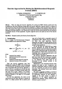
frequently used notations for algorithm analysis are the Ω notation and the Θ notation. The Ω notation provides an asymptotic lower bound, i.e., f (n) is of Ω(g(n)) if there exist positive constants c and n0 such that 0 ≤ cg(n) ≤ f (n), for all n ≥ n0 . On the other hand, the Θ notation provides an asymptotically tight bound for f (n), i.e., f (n) is of Θ(g(n)) if there exist positive constants c1 , c2 and n0 such that 0 ≤ c1 g(n) ≤ f (n) ≤ c2 g(n), for all n ≥ n0 [32]. Figures 2.1(a), 2.1(b) and 2.1(c) demonstrate a graphic example of the O notation, the Ω notation, and the Θ notation respectively.1

(b) The Ω notation

(a) The O notation

(c) The Θ notation

Figure 2.1: Asymptotic Notations.

In addition to analyzing the efficiency of an algorithm, we sometimes need to know what types of algorithms exist for solving a particular problem. The field of complexity analysis analyzes problems rather than algorithms. Two important classes of problems are usually identified in this context. The first class is called P (polynomial time problems). 1

In this thesis we use the O notation for the analysis of algorithms when needed, since it is the most commonly used type of asymptotic notations among the three notations introduced in this section.


14

It contains problems that can be solved using algorithms with running times such as O(n), O(log(n)) and O(nk ) 2 . They are relatively easy problems, sometimes called tractable problems. Another important class is called N P (non-deterministic polynomial time problems). This class includes problems for which there exists an algorithm that can guess a solution and verify whether the guessed solution is correct or not in polynomial time. If we have an unbounded number of processors that each can be used to guess and verify a solution to this problem in parallel, the problem can be solved in polynomial time. One of the big open questions in computer science is whether the class P is equivalent to the class N P. Most scientists believe that they are not equivalent. This, however, has never been proven.

Researchers also distinguish a sub class of N P, called the N P-complete class. In a sense, this class includes the hardest problems in computer science, and is characterized by the fact that either all problems that are N P-complete are in P, or not in P. Many N Pcomplete problems may require finding a subset within a base set (e.g. the SAT problem), or an arrangement (or permutation) of discrete objects (e.g. the TSP), or partitioning an underlying base set (e.g. graph coloring). As mentioned above, these problems belong to the combinatorial optimization class of problems, and sometimes called intractable problems. An optimization problem for which the associated decision problem is N P-complete is called an N P-hard problem. A decision problem is a problem that has only two possible answers: yes or no. For example, if the problem is a cost minimization problem, such that it is required to find a solution with the minimum possible cost, the associated decision problem would be formulated as: “ is there a solution to the problem whose cost is B, where B is a positive real number?”. Figure 2.2 demonstrates how the different complexity classes may relate to each other. For more details about algorithm analysis and complexity theory, the reader is referred to the book by Garey and Johnson [54] and Cormen et al. [32]. Solving CO problems has been a challenge for many researchers in computer science and operations research. Exact methods used to solve regular problems cannot be used to solve CO problems given current resources, since searching among all possible solutions of a certain intractable problem is usually prohibitive for large problem sizes. The natural alternative would be to use approximation methods that give good, rather than optimal, solutions to the problem in a reasonable amount of time. In the next section we briefly consider some exact methods that can be used to solve Running times of O(n) are usually called linear running times. Also, running time of O(nk ) are often referred to as polynomial running times, while running times of O(2n ) are called exponential running times. 2

2.2 Exact Algorithms

15

Figure 2.2: Complexity Classes.

CO problems. However, since exact algorithms are not practical solution methods for the applications considered in this thesis, our discussion of these techniques will be very brief. On the other hand, a more detailed investigation of approximation algorithms, i.e., heuristics and meta-heuristics, will be presented in Section 2.3.

2.2 Exact Algorithms As previously mentioned, exact algorithms are guaranteed to find an optimum solution for a CO problem if one exists, given a sufficient amount of time. In general, the most successful of these algorithms try to reduce the solution space and the number of different alternatives that need to be examined in order to reach the optimum solution. Some exact algorithms that have been applied to solving CO problems are the following:

1. Dynamic Programming (DP): which refers to the process of simplifying a complicated problem by dividing it into smaller subproblems in a recursive manner. Problems that are solved using dynamic programming usually have the potential of being divided into stages with a decision required at each stage. Each stage also has a number of states associated with it. The decision at one stage transforms the current state into a state in the next stage. The decision to move to the next state is only dependent on the current state, not the previous states or decisions. Topdown dynamic programming is based on storing the results of certain calculations, in order to be used later. Bottom-up dynamic programming recursively transforms a

2.3 Heuristic Algorithms

16

complex calculation into a series of simpler calculations. Only certain CO problems are amenable to DP. 2. Branch-and-Bound (B&B): is an optimization technique which is based on a systematic search of all possible solutions, while discarding a large number of nonpromising candidate solutions, using a depth-first strategy. The decision to discard a certain solution is based on estimating upper and lower bounds of the quantity to be optimized, such that nodes whose objective function are lower/higher than the current best are not explored. The algorithm requires a ‘branching’ tool that can split a given set of candidates into two smaller sets, and a ‘bounding’ tool that computes upper and lower bounds for the function to be optimized within a given subset. The process of discarding fruitless solutions is usually called ‘pruning’. The algorithm stops when all nodes of the search tree are either pruned or solved. 3. Branch-and-Cut (B&C): is a B&B technique with an additional cutting step. The idea is to try to reduce the search space of feasible candidates by adding new constraints (cuts). Adding the cutting step may improve the value returned in the bounding step, and could allow solving subproblems without branching.

2.3 Heuristic Algorithms Given the limitation of exact methods in solving large CO problems, approximation techniques are often preferred in many practical situations. Approximation algorithms, like heuristics and meta-heuristics3, are techniques that solve ‘hard’ CO problems in a reasonable amount of computation time, compared to exact algorithms. However, there is no guarantee that the solution obtained is an optimal solution, or that the same solution quality will be obtained every time the algorithm is run. Heuristic algorithms are usually experience-based, with no specific pre-defined rules to apply. Simply, they are a ‘common-sense’ approach to problem solving. On the other hand, an important subclass of heuristics are meta-heuristic algorithms, which are generalpurpose frameworks that can be applied to a wide range of CO problems, with just minor changes to the basic algorithm definition. Many meta-heuristic techniques try to mimic biological, physical or natural phenomena drawn from the real-world. 3

In this discussion we use the term approximation/heuristic algorithm to refer to any ‘non-exact’ solution method. More accurately, however, the term approximation algorithm is often used to refer to an optimization algorithm which provides a solution that is guaranteed to be within a certain distance from the optimum solution every time it is run, with provable runtime bounds [153]. This may not be necessarily the case for heuristic algorithms, though.


17

In solving a CO problem using a heuristic or a meta-heuristic algorithm, the search for a good problem solution is usually divided into two phases: solution construction and solution improvement. Solution construction refers to the process of creating one or more initial feasible solutions that will act as a starting point from which the search progresses. In this phase, a construction heuristic usually starts from an empty solution and gradually adds solution components to the partially constructed solution until a feasible solution is generated. On the other hand, solution improvement tries to gradually modify the starting solution(s), based on some predefined metric, until a certain solution quality is obtained or a given amount of time has passed. Within the context of searching for a good quality solution, we usually use the term search space to refer to the state space of all feasible solutions/states that are reachable from the current solution/state. To find a good quality solution, a heuristic or a meta-heuristic algorithm moves from one state to another, i.e., from one candidate solution to another, through a process that is often called Local Search (LS). During LS, the new solution is usually generated within the neighbourhood of the previous solution. A neighbourhood N(x) of a solution x is a subset of the search space that contains one or more local optima, the best solutions in this neighbourhood. The transition process from one candidate solution to another within its neighbourhood requires a neighbourhood move that changes some attributes of the current solution to transform it to a new solution x′ . A cost function f (x) is used to evaluate each candidate solution x and determine its cost compared to other solutions in its neighbourhood. The best solution within the overall search space is called the globally optimal solution, or simply the optimum solution. Figure 2.3 shows a search space for a minimization function, i.e., our goal is to obtain the global minimum for this function. In this figure three points (solutions) are local optima within their neighbourhoods, A, B and C. The global optimum among the three points is point C. Several modifications to the basic local search algorithm have been suggested to solve CO problems. For example, Baum [10] suggested an Iterated Local Search (ILS) procedure for the TSP, in which a local search is applied to the neighbouring solution x′ to obtain another solution x′′ . An acceptance criterion is then applied to possibly replace x′ by x′′ . Voudouris and Tsang [154] suggest a Guided Local Search (GLS) procedure, in which penalties are added to the objective function based on the search experience. More specifically, the search is driven away from previously visited local optima, by penalizing certain solution features that it considers should not occur in a near-optimal solution. In addition, some local search methods have been formulated under the meta-heuristic framework, in which a set of predefined rules or algorithmic techniques help guide a heuristic


18

Figure 2.3: Search space for a minimization problem: local and global optima.

search towards reaching high quality solutions to complex optimization problems. Among the most famous meta-heuristic techniques are: Hill Climbing (HC), Simulated Annealing (SA), Genetic Algorithms (GAs), Ant Colony Optimization (ACO), Tabu Search and Variable Neighbourhood Search (VNS). For more details about local search techniques and its different variations and applications to CO problems, the reader is referred to [3] and [125]. In what follows we describe some important meta-heuristic techniques that have been widely used for solving CO problems.

2.3.1 Hill Climbing (HC)

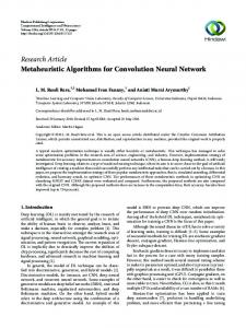
Hill Climbing is the simplest form of local search, where the new neighbouring solution always replaces the current solution if it is better in quality. The process can thus be visualized as a step-by-step movement towards a locally optimum solution. Figure 2.4 shows how an HC algorithm transitions ‘downhill’ from an initial solution to a local minimum. On the other hand, Algorithm 2.1 shows the steps of an HC procedure applied to a minimization problem.


19

Figure 2.4: Hill Climbing: downhill transition from an initial solution to a local optimum.

Algorithm 2.1: Hill Climbing (HC). 1: Generate an initial solution x 2: repeat 3: 4: 5: 6:

Generate a new solution x′ within the neighbourhood of x (x′ ∈ N (x)) ∆ ← f (x′ ) − f (x) if (∆ < 0) then x ← x′

7: until (Done){stopping condition is reached} 8: Return solution x

HC is frequently applied within other meta-heuristic techniques to improve solution quality at various stages of the search. In our research we tried HC among the selected approaches for solving the Single Vehicle Pickup and Delivery Problem with Time Windows (SV-PDPTW), as will be explained in Chapter 6. HC was also an important part of the solution construction heuristics that we developed for the Multiple Vehicle Pickup and Delivery Problem with Time Windows (MV-PDPTW), as will be explained in Chapter 7. We have also applied it in parts of the algorithms developed for solving the One-Commodity Pickup and Delivery Problem (1-PDP), as will be shown in Chapters 9 and 10.

20


2.3.2 Simulated Annealing (SA) Simulated annealing is a well-known meta-heuristic search method that has been used successfully in solving many combinatorial optimization problems. It is a hill climbing algorithm with the added ability to escape from local optima in the search space. However, although it yields excellent solutions, it is very slow compared to a simple hill climbing procedure. The term simulated annealing is adopted from the annealing of solids, where we try to minimize the energy of the system using slow cooling until the atoms reach a stable state. The slow cooling technique allows atoms of the metal to line themselves up and to form a regular crystalline structure that has high density and low energy. The initial temperature and the rate at which the temperature is reduced is called the annealing schedule. The theoretical foundation of SA was led by Kirkpatrick et al. in 1983 [93], where they applied the Metropolis algorithm [107] from statistical mechanics to CO problems. The Metropolis algorithm in statistical mechanics provides a generalization of iterative improvement, where controlled uphill moves (moves that do not lower the energy of the system) are probabilistically accepted in the search for obtaining a better organization and escaping local optima. In each step of the Metropolis algorithm, an atom is given a small random displacement. If the displacement results in a decrease in the system energy, the displacement is accepted and used as a starting point for the next step. If on the other hand the energy of the system is not lowered, the new displacement is accepted with a certain probability exp(−E/kb T ) where E is the change in energy resulting from the displacement, T is the current temperature, and kb is a constant called a Boltzmann constant . Depending on the value returned by this probability either the new displacement is accepted or the old state is retained. For any given T , a sufficient number of iterations always leads to thermal equilibrium. The SA algorithm has also been shown to possess a formal proof of convergence using the theory of Markov Chains [47]. In solving a CO problem using SA, we start with a certain feasible solution to the problem. We then try to optimize this solution using a method analogous to the annealing of solids. A neighbour of this solution is generated using an appropriate method, and the cost (or the fitness) of the new solution is calculated. If the new solution is better than the current solution in terms of reducing cost (or increasing fitness), the new solution is accepted. If the new solution is not better than the current solution, though, the new solution is accepted with a certain probability. The probability of acceptance is usually set to exp(−∆/T ) , where ∆ is the change in cost between the old and the new solution and T is the current temperature. The probability thus decreases exponentially with the badness of


21

the move. The SA procedure is less likely to get stuck in a local optimum, compared to a simple HC, since bad moves still have a chance of being accepted. The annealing temperature is first chosen to be high so that the probability of acceptance will also be high, and almost all new solutions are accepted. The temperature is then gradually reduced so that the probability of acceptance of low quality solutions will be very small and the algorithm works more or less like hill climbing, i.e., high temperatures allow a better exploration of the search space, while lower temperatures allow a fine tuning of a good solution. The process is repeated until the temperature approaches zero or no further improvement can be achieved. This is analogous to the atoms of the solid reaching a crystallized state. Figure 2.5 shows how occasional uphill moves may allow the SA algorithm to escape local optima in a minimization problem, compared to the HC algorithm shown in Figure 2.4.

Figure 2.5: Simulated Annealing: occasional uphill moves and escaping local optima.

Applying SA to CO problems also requires choices concerning both general SA parameters and problem specific decisions. The choice of SA parameters is critical to the performance of the algorithm. These parameters are: the value of the initial temperature T , a temperature function that determines how the temperature will change with time, the

22


number of iterations N(t) to be executed at each temperature, and a stopping criterion to terminate the algorithm. As previously mentioned, the initial temperature T (0) is generally chosen high enough so that almost any move is accepted regardless of its fitness. This choice is adopted from the physical analogy and corresponds to heating up a substance until all particles are randomly arranged in a liquid. The temperature update function is usually a proportional temperature function T (t + 1) = αT (t), where t is the current iteration. Typical values of α lie between 0.8 and 0.99. Using such values provides very small decrements of the temperature, which corresponds to slow cooling of the substance until the temperature approaches zero. The number of iterations carried out at each temperature value should be large enough to bring the system to a stable state equating to thermal equilibrium in the physical analogy. Some applications may choose N(t) to be constant for each temperature. The stopping criterion of the algorithm is usually the stagnation of the system when no change in the result can be obtained for a specified number of iterations or temperature changes. Implementing SA also requires a set of problem-specific decisions. These include: identifying the set of feasible solutions to the problem, defining a clear objective function, generating an initial solution, and defining a neighbourhood operator that generates moves using the current solution. The topology of the neighbourhood structure is also critical to the performance of the SA algorithm. In general, a smooth topology with shallow local optima is favoured over a bumpy topology with many deep local minima. A neighbourhood function is also easy to implement for discrete problems, while implementing a neighbourhood function for continuous problems is more challenging. Constrained problems also raise some difficulties. A choice must be made between restricting the solution space to solutions that conform to the constraints, or allowing solutions that break the constraints at the expense of a suitably defined penalty function. The generic SA algorithm is described in Algorithm 2.2, where the underlying optimization problem is again assumed to be a minimization function. Some modifications to the basic SA algorithm have been suggested. These modifications are intended to provide an improvement of the quality of the solution and/or processing time. One attempt is to store the best solution found so far. Since the SA algorithm accepts solutions probabilistically, it may accept solutions that are worse than the current solution. A good solution found during the run may be discarded because it was not lucky during the acceptance attempt. Storing the best solution found so far prevents the SA algorithm from returning a final solution that is worse than the best solution ever found (e.g. [63]).


23

Algorithm 2.2: The Simulated Annealing (SA) Algorithm. 1: Generate an initial solution x 2: T ← T0 {initialize current temperature} 3: repeat 4: 5: 6: 7: 8: 9:

for (i = 0; i < numIterations; i + +) do Generate a new solution x′ within the neighbourhood of x (x′ ∈ N (x)) ∆ ← f (x′ ) − f (x) if (∆ < 0) then x ← x′

else

10:

p = Random(0, 1) {generate a random number in the interval (0,1)}

11:

if (p < exp(−∆/T ) ) then

12: 13:

x ← x′

T ← α × T {reduce current temperature}


Some researches also modify the basic SA algorithm using problem specific information. For example [148] suggest a neighbourhood operator that is able to identify promising areas in the neighbourhood, and give a greater probability to generated moves that fall in the promising areas. SA has also been hybridized with other optimization techniques. This can be done by using another technique to generate a good initial solution that SA can improve, or using SA to generate a good solution that can be used by another search technique. To sum up, SA has several attractive features, especially in difficult optimization problems in which obtaining a good solution, with a reasonable computational effort and processing time, is preferred to an optimal solution with considerably higher cost. The basic advantages of SA are the following:

1. It is very easy to implement, since it just requires a method for generating a move in the neighbourhood of the current solution, and an appropriate annealing schedule. 2. It can be applied to a wide range of problem types. For example, any combinatorial optimization problem can be tackled using SA, if an appropriate neighbourhood structure has been devised. 3. High quality solutions can be obtained using SA, if a good neighbourhood structure and a good annealing schedule have been chosen.

24


These benefits, however, may be at the expense of a longer processing time, compared to simple hill climbing. In our research we applied SA to solving the SV-PDPTW, as explained in Chapter 6, and for the MV-PDPTTW, as explained in Chapter 8. We also hybridized SA with a Variable Neighbourhood Search (VNS) approach for solving 1-PDP, as will be shown in detail in Chapter 10.

2.3.3 Genetic Algorithms (GAs) The idea of simulation of biological evolution and the natural selection of organisms dates back to the 1950’s. One of the early pioneers in this area was Alex Fraser with his research published in 1957 [50] [51]. Nevertheless, the theoretical foundation of GAs were established by John Holland in 1975 [78], after which GAs became popular as an intelligent optimization technique that may be adopted for solving many difficult problems. The theme of a GA is to simulate the processes of biological evolution, natural selection and survival of the fittest in living organisms. In nature, individuals compete for the resources of the environment, and they also compete in selecting mates for reproduction. Individuals who are better or fitter in terms of their genetic traits survive to breed and produce offspring. Their offspring carry their parents’ basic genetic material, which leads to their survival and breeding. Over many generations, this favourable genetic material propagates to an increasing number of individuals. The combination of good characteristics from different ancestors can sometimes produce ‘super fit’ offspring who out-perform their parents. In this way, species evolve to become better suited to their environment. GAs operate in exactly the same manner. They work on a population of individuals representing possible solutions to a given problem. In traditional GAs, each individual is usually represented by a string of bits analogous to chromosomes and genes, i.e., the parameters of the problem are the genes that are joined together in a solution chromosome. A fitness value is assigned to each individual in order to judge its ability to survive and breed. The highly fit individuals are given a chance to breed by being selected for reproduction. Thus, the selection process usually favours the more fit individuals. Good individuals may be selected several times in one iteration, while poor ones may not be selected at all. By selecting the ‘most fit’ individuals, favourable characteristics spread throughout the population over several generations, and the most promising areas of the search space are explored. Finally, the population should converge to an optimal or near optimal solution. Convergence means that the population evolves toward increasing uniformity, and the average fitness of the population will be very close to the highest fitness. During the reproduction phase of a GA, two individuals breed by combining their genes in


25

an operation called crossover. Not all selected pairs undergo crossover. A random choice is applied, where the likelihood of crossover is some given probability. If crossover is not performed, offspring are produced simply by duplicating their parents. Crossover allows the basic genetic material of parents to pass to their children, who then form the next generation. Another operation that is performed by GAs is mutation. Mutation is applied to each child generated from crossover. With a certain small probability, each gene may be altered. Thus, Crossover allows a rapid exploration of the search space by producing large jumps, while mutation allows a small amount of random search. The basic outline of a GA is shown in the following algorithm: Algorithm 2.3: The Basic Genetic Algorithm (GA). 1: Coding: initialize and encode a random population of solutions called chromosomes 2: repeat 3:

Fitness Assignment: decode and evaluate the fitness of each chromosome

4:

Selection: select some chromosomes from the current population for reproduction, where the selection criterion is based on the fitness of the selected parents

5:

Recombination: with some probability apply crossover between the selected parents to produce new children

6:

Variation: apply mutation with a small probability to some genes of the newly produced offspring, or to selected members of the population

7:

Replacement: integrate the newly generated offspring with the old population to create a new generation

8: until (a certain stopping condition is reached)

The traditional GA uses strings of bits to represent chromosomes. In addition, the classical crossover operator is called one-point crossover, where the two mating chromosomes are each cut once at corresponding points and the sections after the cuts are exchanged. However, many different crossover types have been devised, often involving more than one cut point. For example, in a two-point crossover two cut points are chosen randomly in the parent chromosomes. The section between the selected cut points is exchanged between the two children. Another form of crossover is called uniform crossover, in which a random mask of bits is generated. Each gene in the offspring is created by copying the corresponding gene from one of the parents. The parent is selected according to the value of the corresponding bit in the mask. These three crossover operators are illustrated in Figure 2.6. On the other hand, the most popular mutation operators are point mutation, where one


26

bit in the chromosome is flipped, and inversion mutation, in which a substring is selected at random and the bits within this substring are inverted. Figure 2.7 demonstrates these two mutation operators.

(a) One-point Crossover

(b) Two-point Crossover

(c) Uniform Crossover

Figure 2.6: Crossover.

(a) Point Mutation

(b) Inversion Mutation

Figure 2.7: Mutation.


27

Chromosome representation as a bit string is not suitable for many problems types, though. For example, a permutation of integers representing nodes or locations has been often used for the TSP and other vehicle routing problems. This kind of representation is called an order-based representation, since the fitness depends on the order in which the genes appear. Different crossover and mutation operators must be used in this case, since classical genetic operators, such as the ones described above, will result in ‘infeasible’ chromosomes. Goldberg in [64] described several order-based operators, such as the Partially Matched Crossover (PMX). In a PMX, it is not the genes that are crossed, but the order in which they appear, i.e., offspring have genes that inherit order information from each parent. This avoids the problem of generating offspring that violate problem constraints, such as having duplicate cities in a chromosome that represents a solution to the TSP, or having a chromosome with some non-visited cities. Figure 2.8 shows an example of a PMX, where cities 5,6,7 exchange their positions with 2, 3 and 10 respectively. Other crossover operators that can be used for order-based representations are cycle crossover and order crossover (see [64] for details).

Figure 2.8: Partially Matched Crossover (PMX).

To select two individuals in the population for mating, several selection methods may be applied. For example, in a rank selection, individuals are sorted according to their objective function values, and each individual is assigned a number of offspring that is a function of its rank in the population. Roulette wheel selection picks an individual, with a probability, based on the magnitude of the fitness score relative to the rest of the population. The higher the score, the more likely an individual will be selected, and the probability of the individual being chosen is equal to the fitness of the individual divided by the sum of the fitness values of all individuals in the population. On the other hand, a tournament selection uses the roulette wheel, or another selection method, to select two

28


or more individuals, then picks the one with the higher score. Similarly, many replacement schemes can be used to integrate the new offspring and produce the next generation. In a Simple GA, the new generation of offspring completely replace the old population, while a Steady State GA allows generations to overlap, with a certain percentage of replacement. On the other hand, an Incremental GA only allows a small degree of overlap between generations, for example by replacing one or two individuals at each generation. In summary, GAs represent an intelligent search method, since they operate on a population of solutions and allocate trials to promising areas of the search space. GAs do not depend heavily on information available from the underlying problem. They are easy to connect to existing simulations and models, and can be easily hybridized to generate knowledge-augmented GAs. Using the operations of selection of the fittest, mutation, and crossover, GAs can quickly reach fit individuals (not always the most fit), but who are usually good enough as solutions to problems of a large magnitude. Crossover is considered as the main GA operator. Having to combine two solutions rather than one, makes designing an appropriate crossover operator often more challenging than developing a mutation operator or a simple neighbourhood move. This usually makes GAs implementation more difficult compared to SA or simple HC. In our research we applied GAs to solving the PDPTW, for both the single and multiple vehicle variants, as will be explained in detail in Chapters 5, 6 and 8. We also applied a GA within a perturbation scheme for the 1-PDP, as will be detailed in Chapter 9.

2.3.4 Ant Colony Optimization (ACO) Ant Colony Optimization is a meta-heuristic technique that is inspired by the behaviour of real ants. Its principles were established by Dorigo et al. in 1991 [42]. Real ants cooperate to find food resources by laying a trail of a chemical substance called ‘pheromone’ along the path from the nest to the food source. Depending on the amount of pheromone available on a path, new ants are encouraged, with a high probability, to follow the same path, resulting in even more pheromone being placed on this path. Shorter routes to food sources have higher amounts of pheromone. Thus, over time, the majority of ants are directed to use the shortest path. This type of indirect communication is called ‘stigmergy’ [41], in which the concept of positive feedback is exploited to find the best possible path, based on the experience of previous ants. Figure 2.9 visualizes the foraging behaviour of real ants in their search for food sources.


(a) Two ants start with equal probability of going on either path. The ant on the shorter path arrives more quickly to the food source

(b) The density of the pheromone on the shorter path increases more rapidly than the pheromone on the longer path. Many ants begin using the path with higher pheromone

(c) Over time, the shorter path is almost exclusively used, and the pheromone on the longer path evaporates

Figure 2.9: Foraging behaviour of ants.

29


30

Applying ACO to hard combinatorial optimization problems is attractive, due the flexibility and robustness of the algorithm. In fact, the technique can be applied to solving a wide range of problems with only minimal changes to the basic algorithm. In addition, its population based nature allows exploring the search space, while exploiting positive feedback during the search process to find near optimal solutions. In solving a combinatorial optimization problem using an ACO, the problem may be visualized as finding the shortest path in a weighted graph. Artificial ants (software agents) cooperate to find the best path by constructing solutions consisting of graph nodes stepby-step. Each step adds a selected node to the partial solution in a stochastic manner, but biased by the amount of pheromone available on the nodes or the edges connecting them. To this end, problem-specific information is placed in a common memory, which plays the role of the pheromone trail. The information in the memory, i.e., the pheromone trail, is updated by ants at each iteration, allowing ants to cooperate in finding good problem solutions. Pheromone values also diminish over time, similar to the evaporation of real pheromone. Thus, solutions of bad quality are eliminated from further consideration as the search progresses. Algorithm 2.4 shows the main steps of the ACO meta-heuristic. Algorithm 2.4: The Ant Colony Optimization (ACO) Algorithm. 1: Set parameters, initialize pheromone trails 2: while (termination condition not met) do 3:

ConstructAntSolutions

4:

DaemonActions {optional}

5:

UpdatePheromones

The steps of Algorithm 2.4 are briefly explained below: 1. ConstructAntSolutions: during this phase, each ant constructs a solution from the set of feasible problem solutions, by adding one solution component at each step of the construction process to the current partial solution. For example, in solving a TSP, the construction process will add one non-visited city at a time to the current solution. The choice of the new solution component depends on a probabilistic rule that takes into account both the pheromone trail of the component at the current iteration and other problem-specific heuristic information. In a TSP, the pheromone trail is associated with the edge connecting the last added city and the potential new city, such that edges previously used by other ants are favoured, due to an increased pheromone value. On the other hand, the heuristic information (sometimes called the attractiveness) will be proportional to the length of the edge connecting the two


31

cities. Certain parameters are also used in the probabilistic rule to determine the relative importance of the pheromone trail and the heuristic information. During the solution construction, individual ants may update the pheromone trail on the edges they visited in a process called local pheromone update. 2. DaemonActions: in this optional step of the ACO algorithm, some problem-specific action may be required, which cannot be usually performed by a single ant. For example, local search may be applied to optimize the set of generated solutions. The new optimized solutions are then used to decide which pheromone trails to update. 3. UpdatePheromones: this is a global pheromone update process that is performed at the end of each iteration, where updating the pheromone values depends on the quality of the generated solutions in the current iteration. This is usually done by decreasing the pheromone value for all solutions, in a process called evaporation, and increasing the pheromone value of good solutions. Evaporation is a tool that ACO uses to explore new areas of the search space and avoid being trapped in local optima. ACO has become very popular in solving CO problems. For example, its versatility and robustness have been demonstrated in [43] by tailoring the approach to the TSP, the asymmetric TSP, the Quadratic Assignment Problem (QAP), and the job-shop scheduling. It has also been applied to variants of vehicle routing problems (e.g. [39] and [90]). The idea of ‘attractiveness’ and ‘pheromone trails’ were also exploited within other meta-heuristic techniques. For example, in the crossover operator used by [158] for solving the 1-PDP. For further information about the various types of Ant systems and their applications, the reader is referred to the book by Dorigo and Stützle [44].

2.3.5 Tabu Search (TS) Tabu search is another popular search technique proposed by Glover in 1977 [59]. Since then, it has been widely used for solving CO problems. Its name is derived from the word ‘taboo’ meaning forbidden or restricted. TS, like SA, allows for exploring the search space ‘intelligently’ in an attempt to escape the trap of local optima. Nevertheless, there are three main differences between TS and SA. Firstly, unlike SA, TS only accepts moves within the vicinity of the current solution that improve the objective function. Secondly, TS always searches for the best solution in the current neighbourhood before applying the replacement criterion. Thirdly, the most distinguishing feature of TS is the use of


32

a short term memory called a tabu list, in which moves that have been recently visited during the search are recorded. Moves in the tabu list are considered prohibited by the search and cannot be visited again for a certain number of iterations. The idea is to avoid the problem of cycling, meaning that the search may be trapped within the boundaries of a certain neighbourhood region, oscillating among solutions that have been previously visited, as illustrated in Figure 2.10. By prohibiting recently visited moves, the algorithm is forced to explore new areas of the search space in an attempt to escape local optima.

Figure 2.10: The problem of cycling.

The size of the tabu list is usually fixed, such that some old tabu moves are removed to allow for recording new moves recently visited, and the duration that a move is declared tabu is called its tabu tenure. Hence, the structure of the neighbourhood being searched varies dynamically from one iteration to another. However, always restricting the search to non-tabu moves may prevent some promising search areas from being explored. To avoid this problem, TS often makes use of an aspiration criteria, which allow overriding the tabu status of some moves that look attractive from a search perspective. For example, an aspiration criterion may override the tabu status of a newly generated solution, if its objective value is better than the best solution found so far. To determine the tabu status of certain solutions, it is common in tabu search to identify particular solution features or neighbourhood moves as ‘undesirable’. Accordingly, a newly generated solution holding such features will be considered tabu. Similarly, some


33

previously identified tabu moves may be prohibited during certain stages of the search. Algorithm 2.5 shows the main steps of TS for a cost minimization problem. Algorithm 2.5: The Tabu Search (TS) Algorithm. 1: Initialize an empty Tabu List T 2: Generate an initial solution x 3: Let x∗ ← x {x∗ is the best so far solution} 4: repeat 5:

Generate a subset S of solutions in N (x) {N (x) is the current neighbourhood of x}

6:

Select the best neighbourhood move x′ ∈ S, where f (x′ ) < f (x)

7: 8:

if (f (x′ ) < f (x∗ )) then

x∗ ← x′ {aspiration condition: if current solution improves best so far, accept it even if

it is in the tabu list} 9: 10: 11: 12: 13: 14: 15: 16:

x ← x′ {update current solution} T ← T + x′ {update tabu list}

else

if (x′ ∈ N (x) \ T ) then

x ← x′ {update current solution if the new solution is not tabu} if (f (x′ ) < f (x∗ )) then

x∗ ← x′ {update the best so far solution if the new solution is better in quality}

T ← T + x′ {update tabu list}

17: until (Done){stopping condition is reached} 18: Return solution x∗

It is also sometimes fruitful in TS to make use of an intensification and/or a diversification mechanism. Intensification tries to enhance the search around good solutions, while diversification tries to force the algorithm to explore new search areas, in order to escape local optima. For example, intensification can be performed by encouraging solutions that have some common features with the current solution. On the other hand, diversification may be enforced by applying a penalty in the objective function, at some stage of the search, to solutions that are close to the present one [156]. Some variations of TS also exist in the literature, for example Probabilistic TS assigns a probability to neighbourhood moves, such that some attractive moves that lower the solution cost are given a higher probability, while moves that result in a repetition of some previous state are given a lower probability [63]. Also, a Reactive TS was proposed by Battiti and Tecchiolli [8] in which the size of the tabu list is adapted dynamically during the search, according to the frequency of repeated moves. TS has been extensively applied to many CO problems. For example, it has been applied


34

to scheduling in manufacturing systems in [113], to uniform graph partitioning in [36], to the Quadratic Assignment Problem (QAP) in [140]. In addition, it was applied to many variants of vehicle routing problems, for example in [129], [100], [112], [143] and [99]. For more details about some variations and applications of tabu search, the reader is referred to [62] and [55].

2.3.6 Variable Neighbourhood Search (VNS) Variable Neighbourhood Search (VNS) is a relatively new meta-heuristic that has been suggested by Hansen and Mladenovi´c in [69] and [70]. The main idea is based on exploring the search space by gradually increasing the neighbourhood size, within which a new solution is generated, until a certain stopping condition is reached. In addition, whenever a new solution is generated in the current neighbourhood, a local search is applied to this solution to optimize it before the replacement decision is undertaken. The basic VNS algorithm, as described in [70], is shown in Algorithm 2.6. Algorithm 2.6: The Variable Neighbourhood Search (VNS) Algorithm [70] . 1: Initialization: Select the set of neighbourhood structures Nk , (k = 1, ...kmax ), that will be

used in the search 2: Generate an initial solution x 3: repeat 4: 5:

k←1

while (k < kmax ) do

6:

Shaking: Generate a point x′ at random from the kth neighbourhood of x (x′ ∈ Nk (x))

7:

Local Search: Apply some local search method with x′ as initial solution; denote with x′′ the so-obtained local optimum

8:

Move or not: if the local optimum x′′ is better than the incumbent, move there (x ← x′′ ),

and continue the search with N1 (k ← 1); otherwise set k ← k + 1


In the above VNS algorithm, the neighbourhood size k increases from 1 to a certain maximum value kmax . The most important step is the Shaking step in which a new point (solution) is generated within the current neighbourhood Nk (x). It is crucial to choose a shaking procedure that will allow enough perturbation of the solution, while preserving, at the same time, the most favourable solution features which should be utilized in obtaining


35

a near optimum solution as the search progresses. For example, in solving the TSP, shaking my be performed by displacing or inverting a sequence of k cities in each iteration, i.e., the number of cities to be displaced is the variable neighbourhood size that gradually increases from one iteration to the next. On the other hand, the local search step in the VNS algorithm intensifies the search to obtain a local optimum, which may replace the current solution. For example, in a TSP a 2-Opt improvement heuristic may be applied as a local improvement method (see Section 3.4 for more details about the 2-Opt heuristic). The basic VNS procedure is a descent algorithm with a first acceptance criterion. However, the algorithm can be easily changed to a descent/ascent procedure, similar to SA, by accepting bad moves with a certain probability in Step 8 (move or not) of Algorithm 2.6. Also, the first improvement criterion adopted by the basic VNS in the same step, may be changed to a best improvement by selecting the neighbourhood k ∗ , which yields the best improvement, among all kmax neighbourhoods. Other variations include starting the neighbourhood size from a certain value kmin rather than 1, and varying the step size, such that increasing the neighbourhood size allows jumps to far away regions of the space [70]. Another important variant of the basic VNS algorithm, called Variable Neighbourhood Descent (VND), was also suggested by Hansen in [70]. The idea is to apply a change of neighbourhood size within the local search as well. The steps of the VND algorithm as described in [70] are shown in Algorithm 2.7. Algorithm 2.7: The Variable Neighbourhood Descent (VND) Algorithm [70] . 1: Initialization: Select the set of neighbourhood structures Nk , (k = 1, ...kmax ), that will be

used in the local search 2: Generate an initial solution x 3: repeat 4: 5: 6: 7:

Set k ← 1

while (k < kmax ) do Exploration of the neighbourhood: Find the best neighbour x′ of x (x′ ∈ Nk (x)) Move or not: if x′ is better than x, set (x ← x′ ); otherwise set k ← k + 1.

8: until (Done){no further improvement is obtained} 9: Return solution x

The VNS meta-heuristic offers many attractive features that have encouraged researchers to use it for CO problems. First, the algorithm is simple, easy to understand and implement, and, to a large extent, parameter-independent. Second, well-known neighbourhood moves and local search methods can be easily integrated in several ways and applied wi-

36

2.4 Chapter Summary

thin the VNS framework. Third, it is a robust technique that can be used in a variety of problem types with almost no modification to the basic structure of the algorithm. Finally, it can be easily hybridized with other heuristic and meta-heuristic approaches to solve hard optimization problems. In fact, VNS has been successfully used in solving many well-known CO problems. For example, it has been applied to the TSP and the facility location problem in [70], and to the graph coloring problem in [6]. It has also been extensively applied to vehicle routing problems, for example in [19], [119], [118] and [73]. For more details about advances in VNS and its applications, the reader is referred to the recent work by Hansen et al. [71]. As previously mentioned, our research applied the VNS approach, hybridized with SA, in solving the 1-PDP, as will be explained in detail in Chapter 10.

2.4 Chapter Summary Conventional OR techniques may not be sufficient for solving complex optimization problems, which model a large number of decision making strategies in real-world applications. Heuristic and meta-heuristic techniques, which usually perform well in most practical situations, have become increasingly popular among researchers in the optimization field. In this chapter we introduced combinatorial optimization problems and the theory of algorithm and complexity analysis. We then briefly highlighted some exact algorithms that can be used to solve these problems to optimality, for limited problem sizes only. For more practical applications, though, a heuristic or a meta-heuristic approach is usually the preferred option. We reviewed in this chapter some important meta-heuristic techniques like Local Search, Simulated Annealing, Genetic Algorithms, Ant Colony Optimization, Tabu Search, and Variable Neighbourhood Search. In the next chapter, we will introduce an important class of CO problems, which is the class of vehicle routing and scheduling. A particular variant of vehicle routing problems, pickup and delivery problems, is introduced in Chapter 4. Since pickup and delivery problems are the main theme of our research, our investigation of some selected problems from this category continues in Chapters 5 to 10.

37

Chapter 3

Vehicle Routing Problems: A Literature Review Solving the Vehicle Routing Problem (VRP) and its related variants is an important field in the area of Operations Research (OR), which has attracted a growing interest in recent years. Effective decision support tools that can be adopted in logistic planning are currently in great demand, since they can lead to a substantial cost reduction and efficient resource consumption. In addition, they can help reduce the negative environmental impacts of transportation. An European Commission White Paper [1] states: A modern transport system must be sustainable from an economic and social as well as an environmental viewpoint. Plans for the future of the transport sector must take account of its economic importance. Total expenditure runs to some EUR 1000 billion, which is more than 10% of gross domestic product. The sector employs more than 10 million people. It involves infrastructure and technologies whose cost to society is such that there must be no errors of judgment.

The use of automated route planning and scheduling can lead to huge savings in transportation costs, typically ranging from 5% to 20% [147], which should contribute to boosting the overall economic system. This great potential, together with the advancement in technological and computational powers in the last three decades, has encouraged researchers to experiment with diverse algorithms and address different applications, in order to meet the increase in demand for effective vehicle routing support tools. This indeed resulted in a large increase in the literature dealing with the VRP, especially given that its theme encompasses several intertwined disciplines, such as scientific computing, operations research, and business and management [48]. The rest of this chapter is organized as follows: Section 3.1 gives an idea about the different types of vehicle routing problems existing in the literature and highlights the diversity of published research in this area. Section 3.2 briefly describes one particular VRP variant that is of interest to our research: the Vehicle Routing Problem with Time Windows

38

3.1 Vehicle Routing Problems (VRPs)

(VRPTW). Section 3.3 emphasizes heuristic approaches for the solution construction of the VRPTW, while Section 3.4 describes some popular solution improvement heuristics. Section 3.5 then briefly summarizes some meta-heuristic algorithms that were applied to the VRPTW. Finally, section 3.6 concludes this chapter with a short summary.

3.1 Vehicle Routing Problems (VRPs) VRPs generally involve problems that deal with the transportation of goods or people between depots and customers, where the objective is to design an optimum schedule for one or more vehicles to service the clients with minimum possible operational cost and maximum customer satisfaction. For example, the routing and scheduling plan may try to minimize the number of vehicles used, the total distance traveled, and the labour force used. At the same time, it may try to maximize orders and volumes serviced per unit distance. Moreover, for practical applicability of the problem, a number of constraints are usually added to the basic model. These may include respecting the capacity of the vehicle, applying a certain visiting order, or adhering to preferred service times for clients and to the maximum working hours of drivers. Other practical considerations include service types for customers (delivery and/or collection), number of depots (one/two/multiple), types of operating vehicles (homogeneous/heterogeneous), drivers availability (fixed/variable start times), and whether the information concerning routing requests is known in advance or revealed in real-time. As a generalization of the famous TSP, the VRP is an N P-hard problem [54] [147]. This

fact, together with the above mentioned constraints and practical considerations, add to the difficulty of handling the different variants of vehicle routing problems, and contribute to the existence of a wealth of models and algorithms that deal with this problem. Given the large amount of published research tackling the various types of VRPs [48], it becomes increasingly difficult to keep track of all problem types and underlying solution methods. However, a general classification of the basic routing and scheduling problems and their interconnections is shown in Figure 3.1. Two main problem categories are distinguished in this figure, based on the observation that routing and scheduling problems are usually represented as graphical networks, in which pickup and/or delivery points are represented as nodes connected with line segments called arcs. The first category is called node routing problems, in which the service demand is associated with nodes (locations). The second category is called arc routing problems, in which the service demand is associated with the arc connecting two nodes. Arc routing problems involve applications like refuse collection and winter gritting, and are often referred to as


39

the Chinese Postman Problem (CPP) [66]. The CPP, though, is beyond the scope of our research and will not be addressed further. As Figure 3.1 indicates, the simplest type of node routing problems is the TSP, in which a single vehicle is required to visit a number of nodes, with no restriction on the capacity of the vehicle. It is required in the TSP that the trip starts and ends at the same node, without identifying a particular depot point. The multiple-vehicle variant of the TSP is called the Multiple Traveling Salesman Problem (MTSP). If the demands of locations are added to the problem, the capacity of the vehicle is restricted, and a depot point is identified, it is usually called the Capacitated Vehicle Routing Problem (CVRP). Requesting two different service types (pickup and delivery) in the problem instance, transforms it to the Pickup and Delivery Problem (PDP) category. In addition, a service time window (TW) may be imposed on any of the above variants to allow for more realistic applications of the problem, in which the visiting time of each node is restricted between certain pre-defined bounds. For further details about the main variants of the VRP and both exact and heuristic methods applied to solving it, the reader is referred to the book edited by Toth and Vigo [147].

Figure 3.1: Vehicle routing and scheduling problems.


40

Recently, Eksioglu et al. in 2009 carried out a taxonomic review of the VRP [48], in which they demonstrated that the growth in the literature published from 1955 to 2005 is almost perfectly exponential, if we eliminate the first two years of data. Despite this large increase in published VRP literature, other OR/MS (Operations Research/Management Sience) disciplines have grown at a much higher rate, which indicates that research in the VRP area is probably more sophisticated and requires high skills in analysis and design. The authors classified the characteristics of different VRPs, which should help understand the extent of the available literature and also identify potential areas where more research seems to be needed. Their taxonomy of the VRP research as it appears in [48] is shown in Figure 3.2. This taxonomy classifies the VRP literature under five major categories: 1. Type of Study: which identifies the nature of the study itself, for example: theoretical or applied. Some techniques listed under applied literature include exact and heuristic methods. 2. Scenario Characteristic: which indicates the problem characteristics and the operating scenario of the vehicle routing process. For example, under this category, static problems, in which all requests are determined in advance of the solution process, are distinguished from dynamic problems in which some requests may arrive later (in real-time). Dynamic problems should account for some probable changes in the current progressing routing plan. Other problem characteristics identified here include the type of service (pickup/delivery), and the precedence and coupling requirements 1 . 3. Problem Physical Characteristics: which outlines factors that directly affect the solution, such as number of depots, number of vehicles, capacity and time windows constraints. This category also distinguishes node routing problems from arc routing problems. 4. Information Characteristics: which identifies the nature of information presented and accessed by the underlying solution methodology, and is mainly directed to the study of fuzzy and dynamic routing problems. For example, acting under uncertainty, when certain information (e.g. delays/vehicle breakdown) are revealed during an emergency situation, may fall under this category. 5. Data Characteristics: identifies the type of data used to evaluate the solution method, such as real-world or synthesized data. 1

Precedence means that a pickup location must precede its corresponding delivery, while coupling requires that both the pickup and its delivery must be served by the same vehicle.


Figure 3.2: Taxonomy of the VRP literature [48].

41

42

3.2 The Vehicle Routing Problem with Time Windows (VRPTW)

The above taxonomy gives a general idea about how sophisticated and diverse the VRP literature is. As previously mentioned in the introduction to this thesis (Chapter 1), our research mainly focuses on one particular variant of vehicle routing problems, which are problems that deal with two types of services simultaneously, pickup and delivery (PD). Specifically, we selected two main problems from this category, the Pickup and Delivery Problem with Time Windows (PDPTW) and the One-commodity Pickup and Delivery Problem (1-PDP), with more emphasis on the first of these two variants. In the next chapter, we will present a brief summary of some important PD problems, and give examples of published research in this field. On the other hand, we will devote the rest of this chapter to an important and closely related problem in the literature, which is the Vehicle Routing Problem with Time Windows (VRPTW). This problem is significant to our research, because it bears similarities to our selected PD problems, in terms of the constraints involved and the solution approaches used, as well as the objective function. Moreover, it is one of the most well-studied problems in the vehicle routing field. As previously mentioned in Chapter 2, exact algorithms have their limitations in solving large scale combinatorial optimization problems. In the vehicle routing domain, Hasle and Kloster [72] indicate that today’s exact methods cannot consistently solve VRP instances having more than 50-100 customers, which is generally small for most realistic applications. Moreover, given the complexity of the problem, it is very unlikely that an algorithm that solves the problem to optimality in a reasonable time will be developed in the near future. Hence, our research mainly investigates heuristics and meta-heuristics as possible solution methods to the problems of interest. This literature review will, therefore, focus on the approximation techniques introduced in Chapter 2. In other words, we will highlight selected published research that deals with heuristic and meta-heuristic methods only. Information about research that uses exact methods can be found in several vehicle routing and pickup and delivery problems surveys that we are going to mention throughout this discussion . In this chapter and the next chapter, a general classification and overview of the literature is presented, while more details about previous research particularly related to the individual problems we tackled will be presented in the chapters dedicated to these problems (i.e., Chapters 5 to 10).

3.2 The Vehicle Routing Problem with Time Windows (VRPTW) The VRPTW is an important problem occurring frequently in transportation systems. The problem deals with a number of customer requests that must be dealt with by a fleet of

3.2 The Vehicle Routing Problem with Time Windows (VRPTW)

43

vehicles. All customers are assumed to require the same type of service (either pickup or delivery but not both) 2 . Each vehicle route must start and end at a central depot, and each customer must be visited exactly once. Two main constraints are strictly enforced in this problem. The capacity constraint requires that the vehicle capacity should not be exceeded at any time, while the time window (TW) constraint requires that each customer must be visited during a pre-specified time window interval, i.e., if the vehicle reaches the customer before the beginning of its TW, it should wait until the allowed service time begins. Similarly, arrival after the deadline of the TW means a violation of problem constraints. The solution objective is usually hierarchical, such that the minimization of the number of vehicles used is a primary objective, followed by minimizing the total travel distance of the operating fleet, or the total schedule duration. Figure 3.3 shows a representation of a small instance of the VRPTW, before solving it (Figure 3.3(a)) and after solution (Figure 3.3(b)).

(a) VRPTW - before solution

(b) VRPTW - after solution

Figure 3.3: The vehicle routing problem with time windows.

The VRPTW is one of the most well-studied problems in the vehicle routing research. Both exact and heuristic methods have been widely applied to solving this problem. In our current literature summary, we mostly base our review on the 2-part survey of the VRPTW by Bräysy and Gendreau [20] and [21]. As previously mentioned, our investigation of the problem focuses on heuristic and meta-heuristic solution methods, since exact methods are only limited to small problem sizes. Up-to-date exact algorithms were only capable of solving some of Solomon’s benchmark instances (developed in [141]) of 100 customers 2

In the current discussion, we use the terms requests and customers interchangeably to refer to the set of nodes to be visited. Nevertheless, a distinction between the two terms will be introduced within the context of the PDPTW in Chapters 5 to 8.

44

3.3 Solution Construction for the VRPTW

to optimality. Moreover, most of the solved instances are characterized by having a short schedule horizon (a short TW width). The remaining (unsolved) instances have a long schedule horizon, and are much harder for exact algorithms to solve. For further details about some important exact algorithms in the VRPTW literature, the reader is refereed to Cordeau et al. [28]. Solving the VRPTW generally requires two types of decisions: 1) the assignment or the grouping decision, which means to assign to each vehicle a subset of nodes from the customers set, and 2) the routing and scheduling decision which involves generating a minimum cost route for each vehicle to visit its assigned requests, such that the generated route respects the capacity and TW constraints. It is often observed that for vehicle routing problems of this sort, the assignment decision is usually of more importance than the routing and the scheduling decision, in determining the final solution quality [137]. In addition, the solution process often consists of two phases: solution construction, in which one or more solutions for the problem is generated, and solution improvement, in which the initial solution is improved using a heuristic or a meta-heuristic approach. Both phases are discussed in the following two sections.

3.3 Solution Construction for the VRPTW Solution construction refers to the creation of a set of routes for the vehicles by selecting nodes (customers) and inserting them in one of the partial routes already created, or in a new route. The decision to select a particular node for insertion is usually based on a cost-minimization criterion, and requires that the insertion of the node in a selected route does not cause violations of problem constraints. Two main types of solution construction exist in the VRPTW literature: sequential construction, which builds routes one after the other, and parallel construction which builds several routes at the same time. Sequential construction does not attempt to allocate an additional vehicle unless no more requests can be ‘feasibly’ added to the current vehicle. A parallel construction, on the other hand, initially pre-specifies the number of vehicles that could be used, but more vehicles can be added as needed if the initial estimate of the number of vehicles does not serve all requests without violating the constraints of the problem. Figure 3.4 demonstrates these two variants.


(a) Sequential construction

45

(b) Parallel construction

Figure 3.4: Solution Construction.

Several famous construction heuristic are described by Solomon in [141]. These are the savings heuristics, the time oriented nearest neighbour heuristic, the insertion heuristics, and the time oriented sweep heuristic. These heuristics are briefly explained below.

3.3.1 Savings Heuristics This method is based on one of the most successful construction heuristics for the VRP, the savings heuristic proposed by Clarke and Wright [26]. The idea is to initially assign each customer individually to one vehicle. Thus, an initial vehicle route will only consist of a trip from the depot to the customer and then back to the depot. If we have two such routes, one serving customers i and another serving customer j, combining the two routes such that the new route will service both i and j will result in a saving of service cost Sij = ci0 + c0j − cij . This idea is illustrated in Figure 3.5. The parallel savings construction algorithm for the VRPTW can be summarized as follows: 1. Step 1: compute saving Sij for every two customers i and j, and sort them from largest to smallest; 2. Step 2: take saving Sij from top of the saving list. Search for a route containing (0, i) and another containing (j, 0). If such routes exist, join them to form route (0, i, j, 0). Solomon in [141] adapted the Clarke and Wright savings heuristic to the VRPTW by taking the route orientation into account, as shown in Figure 3.5 and Step 2 above. In addition the algorithm must check the capacity and time window feasibility at every step


46

Figure 3.5: The savings heuristic.

in the heuristic process 3 . A limit on the waiting time is also imposed when routes are joined. A sequential version of the savings heuristic will consider one route at a time, and then implement the best saving that can be achieved if another route is joined with the current route. The sequential savings heuristic can be briefly described as follows: 1. Step 1: compute saving Sij for every two customers i and j, and sort them from largest to smallest; 2. Step 2: consider the current route (0, i, ..., j, 0). Find routes containing (k, 0) and (0, l) that have the best savings Ski and Sjl in the saving list, and select the best one among them for joining with the current route. If no more savings can be implemented for the current route, move to the next route.

3.3.2 Time Oriented Nearest Neighbour Heuristic This heuristic is a sequential construction process that starts by initializing the current route with the depot. Then the customer closest to the depot, in terms of a certain cost measure c, is inserted next in the route. Subsequently, the customer ‘closest’ to the last added customer will be inserted next, if its insertion causes no constraint violation. If 3

Solomon also proposed an important heuristic for speeding the TW feasibility checking called the push forward (PF) heuristic, which is based on calculating the extra time occurring in the schedule due to the insertion of the new node in the route. For more derails see [141].


47

all remaining un-routed customers cannot be feasibly inserted in the current route, a new route is allocated and the process is repeated. The cost function c used by Solomon in [141] to determine the ‘closeness’ between two customers, is based on both geographical and temporal separation between the two nodes. This measure is described by cij = w1 ×dij + w2 ×Tij + w3 ×vij , where dij is the distance between the two customers4 , Tij is the time difference between the completion of the service at i and the beginning of the service at j, and vij is the urgency of visiting customer j, which is calculated as the time remaining until the deadline of servicing customer j is reached. The weights w1 , w2 and w3 satisfy: w1 + w2 + w3 = 1.0, and w1 ≥ 0, w2 ≥ 0 and w3 ≥ 0.

3.3.3 Insertion Heuristics This is another class of sequential construction heuristics described by Solomon in [141], and is based on expanding the current route by inserting one un-routed customer at each iteration. The general idea is demonstrated in Figure 3.6, where the un-routed customer k (left) was inserted between customers i and j (right) in the progressing route.

Figure 3.6: The insertion heuristic.

More specifically, the insertion heuristic starts by initializing the route under consideration with a seed customer. Other customers are then selected for addition to the current route, 4

One simplifying assumption that is usually made in the VRP is that the speed of the vehicle is constant (often = 1). If this assumption is made, the distance separating i and j (dij ) and the travel time between i and j (tij ) may be used interchangeably.


48

based on two cost measures to be defined shortly. When no more un-routed customers can be ‘feasibly’ inserted in the current route, the process is repeated for a new route. The seed customer could be selected as the customer farthest from the depot, or as the customer having the earliest allowed starting service time. Three insertion heuristics have been defined by Solomon, based on the criteria used for selecting an un-routed customer to be inserted next in the current route. The first and most successful insertion heuristic (called I1 insertion) proceeds as follows, after initializing the route with a seed customer: 1. Assume the current partial route created is (i0 , i1 , i2 , ...im ), where i0 and im represent the depot; 2. For each un-routed customer u, find its best feasible insertion position in the route, between two adjacent customers i and j. The best insertion position is the one that minimizes the first cost measure, which we will call c1 (u). c1 (u) is a measure that is calculated based on both the extra travel distance and time delay that happens in the route, due to the insertion of u; 3. Find the best customer u∗ to be inserted in the route, where u∗ is the customer having the maximum value of a second measure, which we will call c2 (u). c2 (u) is calculated based on both c1 (u) (the first measure) and the distance from the depot. The second insertion heuristic (I2) differs from I1 in the definition of the measure c2 (u), since it is now a combined measure of the total route distance and time resulting after the insertion of u (rather than the extra distance and time, as in I1). On the other hand, the third sequential insertion heuristic (I3) differs from I1 in the definition of c1 (u), since the urgency of servicing the new customer u is now also considered in this measure5 . These insertion heuristics are in fact a generalization of the time oriented nearest neighbour heuristic, described in Section 3.3.2, since they allow for inserting a new customer between any two nodes in the route, rather than only at the end. They are sometimes referred to in the literature as the cheapest insertion heuristics, with I1 being the most popular among them. A parallel construction heuristic for the VRPTW was proposed by Potvin and Rousseau [121], based on the I1 heuristic described above. In this heuristic several routes are first initialized with seed customers. To determine the number of initial routes, the authors 5

Our presentation of Solomon’s insertion techniques and the cost measures adopted within these heuristics is simplified to a large extent, in order to fit the general overview intended here. For further information, the reader is referred to [141] and [20].

3.4 Solution Improvement for the VRPTW

49

first ran the I1 sequential construction algorithm. Further routes are later added as needed if the initial number of routes does not yield a feasible solution. After determining the best (feasible and least cost) insertion position for each un-routed customer, the customer whose insertion in the solution causes the least increase in the overall cost is selected next for insertion. Besides a weighted sum of the extra travel distance and time delay used by Solomon to determine the cost of the insertion, this parallel heuristic adds a regret measure over all routes. The regret measure is a type of ‘lookahead’ estimate of the cost of not inserting the customer immediately in its current best route, i.e., if its insertion was postponed to be carried out later in a different route. Although these construction algorithms have mainly been designed for the VRPTW, researchers have also adapted them to different problem variants, such as the PDPTW. More discussion about solution construction heuristics from the perspective of the PDPTW will be presented in Chapter 7.

3.3.4 Time Oriented Sweep Heuristic In this heuristic Solomon [141] suggests a two phase approach to construct a VRPTW solution. The first phase is a clustering phase, in which customers are assigned to vehicles in a way similar to the original sweep heuristic suggested by Gillett and Miller [58]. In this heuristic, a centre of gravity is computed based on the angle between the depot and a randomly selected customer. Then, the remaining customers are assigned to vehicles according to the polar angle separating their locations from the centre of gravity. After the assignment phase, the scheduling phase starts by inserting the selected customers in their respective routes, such that the insertion process follows Solomon’s I1 insertion heuristic, explained in Section 3.3.3.

3.4 Solution Improvement for the VRPTW Solution improvement within the context of the VRPTW refers to the gradual and repeated modification of the initial solution until a certain stopping condition is satisfied. The initial solution is usually a feasible solution, obtained using a construction algorithm, such as the ones described in the previous section. One must then define a neighbourhood move that can be applied to the initial/current solution to obtain a new solution within its neighbourhood, i.e., the new solution only differs in a few attributes from the current solution. For example, the new solution could be obtained by modifying some edges connecting customers in the current solution. Afterwards, the generated solution is evaluated based

50

3.4 Solution Improvement for the VRPTW

on the objective function, and may replace the previous solution if it is smaller in cost. Nevertheless, two main acceptance criteria are usually adopted in this context. The first acceptance criterion selects the first solution found in the neighbourhood of the current solution that improves the objective function. On the other hand, the best acceptance examines all solutions in the neighbourhood of the current solution, and selects the best one among them. The above process is often referred to as local search, and usually results in a local optimum that may be very far from the optimal solution. In addition, the quality of the local optimum depends heavily on the quality of the initial solution. Within the vehicle routing literature, edge exchanges are the most popular solution improvement method, first described by Lin [103] for the TSP. Edge exchanges are applied to one route in the current solution, and depend on removing a number k of edges from the current route, and replacing them with another set of k edges. Thus, the process is often called k-exchange. A route that cannot be further improved by a k-exchange is called a k-optimal. Performing all possible k-exchanges on a route requires O(nk ) time. Thus, moves beyond 2 or 3 exchanges are very time consuming. The 2-exchange move is illustrated in Figure 3.7.

Figure 3.7: 2-exchange move.

Several other improvement methods have been described for the VRPTW, a few of them are modifications to the basic edge-exchange moves. We will briefly mention some of the most important methods, without going into details, since most of them are beyond the

3.5 Meta-heuristics for the VRPTW

51

scope of our research. Potvin and Rousseau [122] introduce a modification to the 2-Opt heuristic of [103], called the 2-Opt* exchange heuristic. 2-Opt* works on two different routes (unlike 2-Opt which exchanges edges belonging to the same route). 2-Opt* tries to combine the two routes without changing the orientation of the tours, by appending the last customers of the second route after the first customers of the first route. Also, Or [114] modified the 3-Opt operator of [103] and introduced the Or-Opt operator for the TSP. In this operator, three edges in the original tour are replaced by three new ones without changing the orientation of the tour. Inter-route operators for the VRP were introduced by Savelsbergh [136] and used by Posser and Shaw [123] for the VRPTW. These are the re-locate, exchange and cross operators. The relocate operator moves a customer from one route to another. The exchange swaps two visits in different routes and the cross is similar to the 2-Opt* proposed in [122]. Other neighbourhood operators are the λ-exchange of Osman [115], the CROSSexchange of Taillard et al. [143], the GENI-exchange of Gendreau et al. [56], ejection chains of Glover [60] [61] and cyclic k-transfers of Thompson and Psaraftis [146]. In addition, other improvement heuristics include the Large Neighbourhood Search (LNS) of Shaw [139]. This algorithm removes a large number of customers from their current routes, and re-schedules them at optimal cost. The removed customers could be selected at random, or based on some relatedness measure that takes into account customers demands or starting times. Schrimpf [138] used a similar approach and calls it ruin and recreate. Finally, Bräysy [18] introduces a modified ejection chain approach that also considers re-ordering of the routes. For the interested reader, more details and illustrations of the different types of solution improvement heuristics are presented in [20]. Similar to solution construction approaches, solution improvement methods have also been adapted and applied to PD problems. Some examples of their application to these problems will be presented in the upcoming chapters, when related work to our selected problems is investigated.

3.5 Meta-heuristics for the VRPTW Since our research is particularly focused on meta-heuristic techniques, we highlight in this section some papers that use meta-heuristic approaches for the VRPTW, and explain briefly some important common features among them. Table 3.1 summarizes research

52


that uses Tabu Search (TS), Simulated Annealing (SA), Ant Colony Optimization (ACO), Variable Neighbourhood Search (VNS), and Guided Local Search (GLS). As Table 3.1 indicates, most meta-heuristic techniques apply some cheapest insertion method for the construction of the initial solution, with Solomon’s insertion being the most popular among them. On the other hand, solution improvement is usually performed using well-known neighbourhood moves like 2-Opt, 2-Opt*, 3-Opt, Or-Opt, λinterchange. . . etc. To accelerate the optimization, the search is sometimes limited to neighbourhoods having particular features. For example, in [53] only moves involving arcs close in distance are allowed, while the approach in [22] only considers selected routes and selected customers for merging during the solution construction process. Some approaches allow infeasibility of solutions (e.g. [99]) and penalize the violation in the objective function. In addition, many algorithms apply a specific strategy for reducing the number of vehicles. For example, the algorithm in [53] removes customers from routes having a small number of nodes and inserts them into other routes, using Or-Opt exchanges. Also, in [11] a 2-phase approach is applied, where the first phase is an SA procedure intended to minimize the number of routes, while the second phase focuses on minimizing total distance. On the other hand, the ACO of [52] uses two colonies, one for the minimization of the number of vehicles and the other to minimize total travel distance. Different diversification mechanisms have also been applied within the various metaheuristics to improve solution quality, so that the algorithm is directed towards exploring new areas of the search space. For example, in [129] the search is diversified using an adaptive memory, where routes taken from best solutions found during the search are stored. Some of these routes are combined to form solutions that will act as new starting solutions for the TS. Also, in [143] diversification is applied by penalizing frequently performed exchanges. On the other hand, the approach in [22] adopts a Guided Local Search (GLS) diversification mechanism that penalizes certain solution features, if they are going to bring the search close to previously visited solutions. Intensification of the search around best solutions discovered during the search have also often been considered. For instance, in [101] the SA algorithm is forced to start from the current best solution several times, while the ACO in [52] uses global pheromone updating, to further explore search areas around the best solutions obtained. Also, in [143] intensifying the search is done by selecting the best routes and re-ordering customers within these routes, using Solomon’s I1 insertion. A post-optimization phase is sometimes added to the basic meta-heuristic to further enhance best solutions. For example, the approach in [129] performs a post-optimization


53

using an exact set-partitioning algorithm on routes obtained from the adaptive memory. Also, in [143] the post-optimization technique of [56] is applied to each route of the final solution obtained. In many cases, hybridization of more than one meta-heuristic technique is adopted. For example, in [101] a tabu-embedded SA is used. Also, in [25] the annealing process is enhanced using a varying size tabu-list, and the authors in [11] use both SA and LNS. To complete our review of meta-heuristic techniques for the VRPTW, Table 3.2 summarizes some Genetic Algorithm (GA) approaches that have been applied to this problem. Almost all of these techniques hybridize GAs with some other heuristic, local search, or another meta-heuristic approach for solution construction and/or solution improvement. Solution representation is usually based on integer representation, rather than the classical bit string encoding. Thus, genetic operators are directly applied to problem solutions. The initial population is often created randomly, or by adapting some well known construction methods. For example, in [144], customers are grouped randomly, and then the cheapest insertion method of [65] is used for routing each group of customers. The fitness function is usually based on solution cost, i.e., number of routes, total distance and total duration. However, since some approaches allow violations of problem constraints, the fitness function should take this into account. For example, in [16], the fitness considers the number of un-serviced customers in an infeasible solution. Also, in [15] a penalty is added in the objective function to violated constraints. On the other hand, the selection scheme often applied is roulette-wheel selection. However, other selection methods have also been used. For instance, a ranking scheme is used in [120]. Regarding recombination, most of the GA techniques apply specialized crossover operators, since traditional genetic operators do not usually fit the VRPTW. For example, the authors in [120] propose a Sequence-Based Crossover (SBX) and a Route-Based Crossover (RBX), while the GA in [16] applies special crossover operators that depend on a global precedence relationship among genes, such as the distance or time windows ordering. On the other hand, mutation is often based on traditional local search operators like 2-Opt, 2-Opt*, Or-Opt and LNS. In addition, mutation is sometimes applied to reduce the number of routes in the solution, as in [120] and [15]. To sum up, meta-heuristic approaches to the VRPTW often embed solution construction and improvement methods as described previously. However, they usually obtain better quality solutions than algorithms that apply straightforward solution construction and improvement techniques on their own. This often comes at the expense of greater complexity in implementation and increased computation time, though. Bräysy and Gendreau

3.5 Meta-heuristics for the VRPTW 54

Garcia et al. [53]

Paper TS

TS

Algorithm

Solomon’s insertion

Solomon’s insertion & 2-Opt

Solomon’s insertion

Solution Construction

CROSS

2-Opt, relocate

2-Opt*, Or-Opt

Solution Improvement

Uses adaptive memory containing routes obtained from best solutions visited during the search, with the purpose of providing new starting solutions

Parallel implementation - Only allows moves involving arcs close in distance

Remarks

Table 3.1: Meta-heuristics for the VRPTW.

Rochat and Taillard [129] TS

Li et al. [101]

Chiang and Russell [25]

SA and LNS

Tabuembedded SA

SA

TS

Nearest-neighbour heuristic with probabilistic rules

Not specified

Insertion and extended sweep heuristics of Solomon

The parallel construction of Russell [133]

Relocate from a holding list where all customers are initially stored

CROSS

2-Opt, Or-Opt, relocate, exchange and 2-Opt*

Shifting and exchange of customer segments between and within routes

λ-interchange and k-node interchange

Exchange - relocate

Reducing number of routes using an ejection-chain phase - Second VNS phase for improving total distance

2 colonies: first one minimizes number of vehicles, and the second minimizes total distance - Both cooperate in updating best solution

2-phase approach: SA to minimize number of routes and LNS to minimize total distance

SA restarts from current best solution several times - Reduce routes by reordering customers and inserting them into other routes - Diversification by random shifts and exchange of customer segments

Enhancing of the annealing process via a varying size tabu-list

Allows violation of constraints for a penalty in the objective function - Penalty parameters adjusted dynamically

Taillard et al. [143]

Decomposes solutions into subsets of routes, based on a polar angle associated with the centre of gravity of each route - TS applied to each subset separately - Diversification by penalizing frequently performed exchanges - Intensification by reordering customers within best routes using I1 insertion

Bent and Van Hentenryck [11] ACO

Or-Opt exchanges CROSS-exchanges

Lau et al. [99]

Gambardella et al. [52] VNS

Solomon’s Insertion and the parallel construction of Russell [133]

SPLIT (of routes) - limited CROSS - limited Or-Opt

and

Bräysy [19]

Savings heuristic

Construction algorithm only considers selected routes and selected customers for merging - Initial phase to minimize number of routes, based on simple customer re-insertion - Further improvement using TA & GLS - TA allows local search moves that worsen the objective function, provided it is within a certain threshold limit - GLS penalizes certain solution based on some solution features (e.g. long edges), not considered part of a near-optimal solution

Bräysy et al. [22]

Threshold accepting (TA) & Guided Local Search (GLS)

Exchange a randomly selected portion of the bit string between chromosomes

A set of K seed angles are planted, where K is the number of vehicle. Sector rays are drawn originating from the depot to each seed angle - Routing done using cheapest insertion of Golden and Stewart [65] Chromosome is a problem solution created using Solomon’s cheapest insertion

Solution coded as a permutation of customers - Insertion heuristic used to construct solution Random insertion heuristic - Chromosomes are problem solutions - Two populations: POP1 used to minimize distance and POP2 minimizes constraint violations

Discrete arc-based representation of individuals combined with a binary vector of strategy parameters - Individuals created using greedy insertion from a Restricted Candidate List (RCL), with a probabilistic element

Thangiah [144]

Potvin and Bengio [120]

Blanton and Wainwright [16]

Berger et al. [15]

Repoussis et al. [128]

Multiple-parent recombination applied only to strategy parameters not to problem solutions

Insertion-based crossover (IBX): combining k routes from parent1 (one at a time) with subsets of customers from parent2 - Insertwithin-route crossover (IRNX): simultaneously combines k routes from parent1 with subsets of customers from parent2

Specialized crossover that uses global precedence relationship among customers (TW/distance)

Sequence-Based Crossover (SBX): two sub-tours from two parents are linked together - Route-Based Crossover (RBX) replaces a route of one parent by another route from the second parent - Repair operator applied for infeasible offspring

Crossover

Initial Population

Paper

Mutation rate determined by strategy parameters evolved during the search - Mutation done using “ruin and recreate”

Large Neighbourhood Search (LNS) mutation - Each customer considered for reinsertion in an alternate route. eliminate shortest route - Reorder customers within a route

Randomly exchange 2-edges

Reduce number of routes by inserting customers from a randomly selected short route into another - Local search mutation using Or-Opt exchanges

Randomly change bit value

Mutation

Table 3.2: Genetic Algorithms for the VRPTW.

(λ + µ) Evolution Strategy (ES). Starting from µ individuals, at each iteration a new intermediate population of λ individuals is produced by mutation - Evolutionary search is based only on mutation - Each offspring is further optimized using route elimination and a local search (based on TS) to improve total distance

Simultaneous evolution of two populations (minimize distance & constraint violations) - POP2 has smaller number of routes than POP1 - When a new better solution is obtained from POP2, POP1 is replaced by POP2

The GA searches for a good ordering of customers. while construction of feasible solutions is handled by a greedy heuristic

The approach is named GENEROUS

Cluster first route second approach called GIDEON - Each chromosome is a set of possible clustering scheme and the GA used to improve the clustering - Routes improved by λ-interchange

Remarks

3.5 Meta-heuristics for the VRPTW 55

56

3.6 Chapter Summary

in [21] identified several techniques that seem to give good results when applied within the different meta-heuristic approaches. Some of these techniques are: 1) saving best solutions found during the search, 2) varying the neighbourhood structure, with the size of the neighbourhood being typically small, 3) using a memory structure to facilitate the search, 4) applying a specific strategy for reducing the number of routes in the solution and 5) hybridization of different heuristics and meta-heuristics.

3.6 Chapter Summary Vehicle routing problems have gained considerable attention in the last few decades. This is mainly due to the increase in complexity in transportation and logistics demands, and the urgent need for optimizing client services, reducing operational costs, and limiting the negative environmental impacts that may result from the non-optimal planning of vehicles and their routes. This chapter provided a general classification of vehicle routing problems existing in the literature and highlighted the diversity of problem types, solution methods, and the huge amount of published research that deals with this problem. We emphasized in this chapter one particular vehicle routing problem that is of interest to our study, the Vehicle Routing Problem with Time Windows (VRPTW). This problem is closely related to pickup and delivery problems that we investigated in our research, in terms of: problem definition, solution methods, objective function and constraint handling approaches. We presented in this chapter a summary of some important heuristic and meta-heuristic algorithms that have been applied to solving the VRPTW. The next chapter is devoted to an overview of pickup and delivery problems, which are the main focus of our research. We will present a general classification and highlight some published research in the field, as an introduction to a more in-depth analysis of our selected pickup and delivery problems, which will follow during the course of this thesis.

57

Chapter 4

Pickup and Delivery Problems: A Literature Review We dedicate this chapter to a literature summary of Pickup and Delivery (PD) problems, since they are the main theme of our research. In addition, there are various types of pickup and delivery problems and different classifications of these problems that distinguish them from other variants of vehicle routing problems. PD problems are widely applicable in areas such as: the transportation of raw materials from suppliers to factories, Internet-based pickup from sellers and delivery to buyers, food and beverage collection and delivery, post and parcel delivery, newspaper distribution, and airline and bus scheduling. In addition, an important related variant is the dial-aride problem and the handicapped persons’ transportation, where people instead of goods are transported, giving rise to customer inconvenience issues that should be taken into consideration while constructing a solution. Similar to other vehicle routing problems, pickup and delivery problems have attracted the attention of researchers in the last few decades. Nevertheless, published research tackling these problems is still relatively limited, compared to other variants of vehicle routing problems [137]. Several important surveys of pickup and delivery problems have appeared in the literature. The oldest ones are by Solomon and Desrosiers [142], and Savelsbergh and Sol [137]. Two other surveys appeared recently in [14] and [117]. A survey dedicated to the dial-a-ride problem is in [29]. Another survey on the one-to-one pickup an delivery problems (see Section 4.2 for a description of this problem category) is provided in [31]. In our literature summary, we mostly rely on the information and classification provided by Parragh et al. in 2008 [117], unless otherwise indicated. Parragh et al. [117] classify the different types of pickup and delivery problems under two classes: 1) problems that deal with the transportation of goods from pickup customers (also called backhaul customers) to the depot, and from the depot to delivery customers (also called linehaul customers). This class is called the Vehicle Routing Problem with

4.1 The Vehicle Routing Problem with Backhauls (VRPB)

58

Backhauls (VRPB), and 2) problems that deal with the transportation of goods/people between two pickup and delivery points. This class is called the Vehicle Routing Problem with Pickup and Delivery (VRPPD). Sections 4.1 and 4.2 describe in detail these two categories. Section 4.3 briefly highlights some meta-heuristic techniques that have been applied to pickup and delivery problems. Finally, Section 4.4 concludes this chapter and introduces the rest of the thesis.

4.1 The Vehicle Routing Problem with Backhauls (VRPB) As mentioned above, this class deals with PD problems that involve the transportation of goods from the depot to customers and vice versa. These problems are further subdivided into four categories, generally based on the required visiting order of pickups and deliveries, and whether a customer can demand both types of services. In all cases the objective is to minimize the total cost (e.g. total travel distance) of the routing plan, while adhering to some pre-specified problem constraints. For example, respecting the capacity of the vehicle at all times, and ensuring that the vehicle starts, if needed, with a load that is equal to the total load to be delivered. 1. The vehicle Routing Problem with Clustered Backhauls (VRPCB): where all delivery customers must be visited before all pickup customers. The single vehicle special case of the same problem is denoted by (TSPCB). 2. The Vehicle Routing Problem with Mixed Linehauls and Backhauls (VRPMB): where mixed visiting of pickup and delivery customers are allowed. The single vehicle case of the same problem is denoted by (TSPMB)1 . If the capacity of the vehicle is greater than or equal to the total sum of demands of pickup and delivery customers, the problem coincides with a simple TSP. 3. The Vehicle Routing Problem with Divisible Delivery and Pickup (VRPDDP): where each customer is both a pickup and a delivery customer. In addition, two visits to the same customer is allowed. The single vehicle variant of the same problem is denoted by (TSPDDP). A possible scenario in this variant is that the vehicle could initially visit a few delivery customers to get rid of some of the load it is carrying. Afterwards, the vehicle could visit another set of customers to perform both 1

More details about this problem will be presented in Chapter 9, since this problem is closely related to the One-commodity Pickup and Delivery Problem (1-PDP) that we handled in our research. Nevertheless, we refer to it in our research by the Traveling Salesman Problem with Pickup and Delivery (TSPPD), the name most commonly used for this problem in the literature (e.g. [110] and [75]).

4.1 The Vehicle Routing Problem with Backhauls (VRPB)

59

delivery and collection service at each, and finally a collection service would be performed at customers that were initially visited for delivery. This type of solution is called a ‘lasso’ solution. It is also observed in [117] that a solution method of the VRPMB (the second category) can be applied to the VRPDDP if each customer demanding both delivery and pickup was modeled by two vertices, one for the delivery and another for the pickup. Very little research has been applied to this problem. 4. The Vehicle Routing Problem with Simultaneous Delivery and Pickup (VRPSDP): where each customer demands both a delivery and a pickup, but, unlike the VRPDDP (the third category), only one visit is allowed for each customer. The single vehicle variant is denoted by (TSPSDP). We summarize in Table 4.1 the most important features of the different variants of the VRPB described in this section. In this table, we indicate the problem name, whether the customer is allowed to demand both pickup and delivery, whether delivery customers must all be visited before pickup customers, or otherwise that mixed sequences of visits is allowed. The table also shows whether more than one visit is permitted, and if splitting the demand of one customer is allowed. Finally, the last column of the table gives examples of selected published papers that dealt with the underlying problem, together with the solution method adopted. We used the notations: (LNS) for Large Neighbourhood Search, (TS) for Tabu Search, and (VNS) for Variable Neighbourhood Search. If the paper handled the single vehicle case, we indicate this by (SV) and if it handled the multiple vehicle case, we indicated this by (MV). The authors in [117] concluded from their survey that the LNS algorithm of [132] seems to be the most flexible and accurate meta-heuristic to date, since it can be applied to several problems in the VRPB class, and it provided new best solutions for several benchmark instances. On the other hand, they selected the heuristic in [111] among the fastest algorithms applied to the VRPB.

4.1 The Vehicle Routing Problem with Backhauls (VRPB) 60

Problem

VRPCB TSPCB

Mixed Visiting yes

One Customer Visit

no

Demand Splitting

Example Papers and Solution Methods

Table 4.1: The Vehicle Routing Problem with Backhauls (VRPB). Customer both P&D

Deliveries Visited before Pickups no

Mosheiov [110]- heuristic (SV) Nagy and Salhi [111]- heuristic (MV) Ropke and Pisinger [132]- LNS (MV)

yes

no

Hoff and Løkketangen [77]- TS (SV) Salhi and Nagy [134] - heuristic (MV)

no

yes

Gendreau et al. [57]- heuristic (SV) Thangiah et al. [145]- heuristic (MV) Mladenovi´c and Hansen [108]- VNS (SV) Ropke and Pisinger [132]- LNS (MV)

no (at most two)

no

yes

yes

yes

yes

no

yes

no

yes

no

no

VRPDDP TSPDDP yes

VRPMB TSPMB

VRPSDP TSPSDP

Alshamrani et al. [4]- heuristic (SV) Nagy and Salhi [111]- heuristic (MV) Ropke and Pisinger [132]- LNS (MV)

4.2 The Vehicle Routing Problem with Pickups and Deliveries (VRPPD)

61

4.2 The Vehicle Routing Problem with Pickups and Deliveries (VRPPD) This class refers to problems that deal with the transportation of goods/people between a pickup and a delivery point. Two subclasses can be distinguished in this category: 1. The Pickup and Delivery Vehicle Routing Problem (PDVRP): where pickup and delivery points are unpaired, and one type of commodity is transferred. Thus, pickup customers will supply the demands needed by the delivery customers. The single vehicle variant of this problem is denoted by (PDTSP). The objective function in this problem category is to minimize the total cost of the route(s), without violating the capacity constraints. It should be noted that the PDTSP is the same as the 1-PDP investigated in our research, as explained in detail in Chapters 9 and 10. 2. The Classical Pickup and Delivery Problem (PDP) and the Dial-a-Ride Problem (DARP): where a transportation request is associated with both a pickup (origin) and a delivery (destination), i.e., customers are paired and the demand of the pickup is the same as the demand of its associated delivery. Unlike the PDP, the DARP additionally takes customer inconvenience into account. The single vehicle cases of these problems are denoted by SPDP and SDARP respectively. The objective function for these problems usually tries to minimize the number of vehicles used (in the multiple-vehicle case) as a primary objective, followed by reducing the overall travel distance or service duration. The final solution should also adhere to all underlying problem constraints, such as the vehicle capacity and the visiting time restrictions. Our research handles the PDP problem with the addition of the time window constraint (denoted by PDPTW) in Chapters 5 and 6 for its single vehicle variant (denoted in our research by SV-PDPTW), and Chapters 7 and 8 for its multiple vehicle variant (denoted in our research by MV-PDPTW).

62

4.2 The Vehicle Routing Problem with Pickups and Deliveries (VRPPD)

We provide in Table 4.2 a summary of the most important features pertaining to the VRPPD. We indicate in this table the subcategory name, whether the customers are paired or not, whether a homogeneous commodity or multiple commodities are considered, and whether the problem is primarily associated with the transportation of people or goods. In addition, we highlight the most important constraints that are usually taken into consideration while handling the problem. These include: 1) the precedence constraint, in which a pickup request is required to precede its corresponding delivery, 2) the coupling constraint, which requires that the pickup and delivery pair must be visited by the same vehicle (in case of the multiple-vehicle variant), 3) the capacity constraint, which ensures that the load carried by the vehicle at any given time does not exceed its capacity, 4) the time window constraint, which requires that a customer has to be served in a pre-specified time interval, and 5) the maximum ride time constraint, which ensures that when people are transported, the time they spend in the vehicle does not far exceed the direct travel time between their origin and destination. Finally, the table gives examples of some published papers that deal with the problem. Again, we use (SV) for the single vehicle case and (MV) for the multiple-vehicle variant. (LNS) refers to a Large Neighbourhood Search algorithm, and (ALNS) refers to an Adaptive version of LNS, (HC) is a Hill Climbing approach, (GA) is a Genetic Algorithm, (GGA) is a Grouping Genetic Algorithm, (SA) is a Simulated Annealing algorithm, and (TS) is a Tabu Search algorithm. In our opinion, the GA in [158], the LNS in [12], the ALNS in [131], and the GGA in [126] seem to be among the state-of-the-art algorithms applied to the VRPPD, in terms of their solution quality and/or robustness or flexibility. More details about these approaches and other important research in the field will be described in the following chapters, where we address specific pickup and delivery problems in our research. Before we conclude our review of pickup and delivery problems, though, we present in the next section a brief summary of some meta-heuristic techniques that have been applied to this problem class.

Paired Customers

no

yes

yes

Problem

PDVRP PDTSP

PDP SPDP

DARP SDARP yes

no

yes

One Commodity

people

goods

goods

Type of Commodity

yes

yes

no

yes

yes

no

Precedence Coupling

yes

yes

yes

Capacity

yes

yes

no

TW

yes

no

no

Max Ride Time

Psaraftis [124]- heuristic (SV) Jaw et al. [87]- heuristic (MV) Baugh et al. [9]- SA (MV) Rekiek et al. [126]- GGA (MV) Jørgensen et al. [91]- GA (MV)

Jih and Hsu [89]- GA (SV) Hosny and Mumford [84] - HC & SA & GA (SV) Li and Lim [100]- TS (MV) Bent and Van Hentenryck [12] - LNS (MV) Ropke and Pisinger [131] - ALNS (MV) Hosny and Mumford [80]- GA (MV)

Hernández-Pérez and Salazar-González [75]heuristic (SV) Zhao et al. [158] - GA (SV) Dror et al. [45]- heuristic (MV)

Example Papers and Solution Methods

Table 4.2: The Vehicle Routing Problem with Pickups and Deliveries (VRPPD).

4.2 The Vehicle Routing Problem with Pickups and Deliveries (VRPPD) 63

4.3 Meta-heuristic Algorithms for Pickup and Delivery Problems

64

4.3 Meta-heuristic Algorithms for Pickup and Delivery Problems Similar to all routing and scheduling problems, pickup and delivery problems have attracted the interest of researchers who deal with meta-heuristic techniques, since exact algorithms can only be used for small problem sizes and may not be useful for large practical applications. For example, the approach in [46], for solving the multiple-vehicle PDPTW, was only capable of solving problem sizes of up to 55 customers using an exact algorithm. Also, the exact algorithm in [74], solved PDTSP instances of up to 60 customers. On the other hand, heuristic and meta-heuristic approaches are able to solve problems having several hundreds of nodes, which is common in every day routing and scheduling demands for some industrial applications. For example, Paragon software systems recently reported, in their October 2009 newsletter2, that their optimization software helped Sainsbury’s to manage its transport requirement, involving daily deliveries from 19 distribution centers to 527 supermarkets and 276 smaller stores. Many heuristic and meta-heuristic techniques that have been successfully applied to the VRP have been adapted to fit the PDP variant. Table 4.3 summarizes some meta-heuristic techniques for pickup and delivery problems. In addition to the notations used for the meta-heuristic techniques in Table 4.2, we use (GRASP) for a Greedy Randomized Adaptive Search Procedure, and (VND) for a Variable Neighbourhood Descent algorithm. On the other hand, Table 4.4 summarizes some GA research on pickup and delivery problems. It is important to emphasize again that the review presented here is just intended as a quick introduction to the literature that deals with pickup and delivery problems. As previously mentioned, further investigation of specific work that is closely connected to our research will be presented in later chapters, when we address certain variants of pickup and delivery problems.

2

http://www.paragonrouting.com/cms/assets/pdf/directionsissue22.pdf

PDTSP (SV)

PDPTW (SV)

PDPTW (MV)

PDPTW (MV)

HernándezPérez and SalazarGonzález [73]

Landrieu et al. [95]

Nanry and Barns [112]

Li and [100]

PDPTW (MV)

DARP (MV)

Urban [149]

Cordeau and Laporte [30]

Lim

Problem

Paper

TS

Guided SA

Tabuembedded SA

Reactive TS

TS

Hybrid GRASP & VND

Algorithm

Assigning requests to vehicles randomly and inserting source location followed by destination at the end of the route

Assigning only one pickup and delivery pair to each route. A guided SA is then applied to improve this initial solution by trying to bundle requests into the available routes

Modified Solomon’s insertion heuristic - Initializes each route with a P&D pair that satisfies a set of criteria, based on combined TW intervals and distance from the depot

Cheapest insertion

Simple insertion heuristic

Selecting the next element for insertion from a Restricted Candidate List (RCL), with a probabilistic element in the choice of the next node

Solution Construction

Moving a request from one route to another

Removing a selected request from its current route and inserting it into another - Exchange of requests served on different routes - Repositioning of a pickup and delivery pair in its same route

PD-Shift: moves a P&D pair from route1 to route2, and moves another pair from route2 to route1 - PD-Swap: removes a P&D pair from each route, and then reinserts each pair in the other route - PD-Rearrange: removes and then reinserts a P&D pair in the same route

Single Paired Insertion (SPI): move all predecessor nodes to better feasible locations, then insert successor nodes in the best possible positions - Swapping Pairs Between Routes (SBR): exchange predecessor nodes between vehicles then successor nodes - Within Route Insertion (WRI): re-order nodes within the same route

A swap move and an insertion move

2-Opt and 3-Opt in the VND phase - Move forward and move backward in a post optimization phase

Solution Improvement

Re-insertion of the removed request in its original route is forbidden by for a number of iterations - Diversification penalizes frequently occurring moves in the objective function - Intensification performed by removing all requests from their respective routes, and re-inserting them in the best possible positions

The cost function takes into consideration both wage and non-wage related traveling and operating costs of the vehicles - The selection of neighbourhood move depends on a certain probabilistic criterion - Calculated measurements control the selection of customers and routes during the generation of the new solution

Main meta-heuristic is a tabu-embedded SA with K-restarts, i.e., the algorithm stops when the number of iterations without improvement reaches a pre-defined value K - To prevent cycling, the SA records the accepted solutions in a tabu list

Reactive tabu search - Allows tuning of search parameters, such as a short-term memory length, based on an assessment of visited solutions during the search

Two tabu search methods compared: a regular deterministic Tabu Search (TS), and a Probabilistic Tabu Search (PTS)

Combining two optimization heuristics: 1) GRASP (Greedy Randomized Adaptive Search Procedure), which is based on a repetition of a construction phase and a local search phase, 2) VND (Variable Neighbourhood Descent), which is a variant of the VNS, where the local optimum found acts as the new starting point for the local search

Remarks

Table 4.3: Meta-heuristics for Pickup and Delivery Problems.

4.3 Meta-heuristic Algorithms for Pickup and Delivery Problems 65

4.3 Meta-heuristic Algorithms for Pickup and Delivery Problems 66

Problem

Initial Population

Crossover

3-exchange procedure

Mutation

Initial population is optimized using a 2-Opt move - Pheromone trails are updated each generation - Offspring is optimized using a 2-Opt local search.

Remarks

Table 4.4: Genetic Algorithms for Pickup and Delivery Problems. Paper Nearest-neighbour heuristic

A new pheromone-based crossover - Edges between last node and potential new node that have proved successful in the past are favoured

construction

Zhao et al. [158]

PDTSP (SV)

A solution is encoded as a permutation of locations

A Family Competition Genetic Algorithm (FCGA) - Each individual of the population plays the role of a family father in turn - Another randomly selected individual plays the role of mate for the family father

PDPTW (SV)

Swap two genes selected at random - Select two random sites in the chromosome and reverses the sub-route between them - Shuffle genes that precede a location for which a violation of constraints is observed

Jih and Hsu [89]

Two traditional order-based crossover operators - Two merge crossover operators, MX1 and MX2, that use a global precedence vector to guide the inheritance process, as in [16]

Jung and Haghani [92]

Customers inconvenience is taken into consideration by assigning a penalty in the objective function to the arrival of the vehicle before or after the specified TW

PDPTW (MV)

Two crossover points generated, and the resulting segments swapped between the two parents

traditional GGA crossover as in [49]

Removes a random cluster from a chromosome, and reassigns its requests to other clusters

Change the first digit of a pickup and delivery pair to another digit, i.e., assign the request to another vehicle - Vehicle merging also used to reduce the number of vehicles

DARP (MV)

Vehicles with their assigned requests removed from one parent and inserted in the other parent

Chromosome representation is based on assigning a 4 digit code to each request - First digit represents the number of the vehicle - Remaining 3 digits are used to sort requests according to the visiting order of the vehicle - A pickup request always has a sorting code that is less than its corresponding delivery

al.

A Grouping Genetic Algorithm (GGA), where the GA is only responsible for the grouping (assignment) problem - Routing is handled using an adaptation of Solomon’s cheapest insertion - Chromosome ‘clean up’ needed after the genetic operators to remove duplicate vehicles and repeated assignment of requests, in addition to re-assigning requests that are no longer assigned

PDPTW (MV)

Pankratz [116]

et

A Grouping Genetic Algorithm (GGA) applied to the Handicapped Person Transportation (HPT) problem, which focuses on minimizing clients’ inconvenience - The insertion heuristic used to insert requests in routes is the best-fit (BF) heuristic - An unserved client is inserted in the vehicle that will grant him the best service without violating problem constraints

Each gene represents a group of requests that are assigned to one vehicle - Routes are represented by an independent data structure associated with each gene

Rekiek [126]

Chromosome representation is group oriented, where each group represents a vehicle to which a set of requests is assigned

Create a new group - Remove an existing group - Move items between groups - An inversion operator is also used to change the location of groups in the chromosome

4.4 Chapter Summary

67

4.4 Chapter Summary In this chapter, we reviewed an important category in the VRP literature, which deals with pickup and delivery problems. These problems are gaining more attention every day, due the continuous need for optimizing routing and scheduling costs in real-life applications that require two different service types for clients. We briefly analyzed basic problem features and general existing classifications. We also highlighted some published research in the field, mainly focusing on heuristic and meta-heuristic approaches. In the following chapters, we will start discussing the specific problems that we addressed in our research. The Pickup and Delivery Problem with Time Windows (PDPTW) will be analyzed in detail in Chapters 5 and 6 for its single vehicle variant (SV-PDPTW), and in Chapters 7 and 8 for its multiple vehicle variant (MV-PDPTW). On the other hand, the One-commodity Pickup and Delivery problem (1-PDP) will be thoroughly discussed in Chapters 9 and 10.

68

69

Chapter 5

The Single Vehicle Pickup and Delivery Problem with Time Windows: Introduction and a Genetic Algorithm Approach The Single Vehicle Pickup and Delivery Problem with Time Windows (SV-PDPTW) is a frequently encountered problem in public and goods transport systems. However, only a few researchers seem to have tackled it, possibly due to the difficulty in managing the different underlying problem constraints. As previously mentioned in the introduction to this thesis (Chapter 1), our research concentrates on representational issues and neighbourhood moves within a simple meta-heuristic framework. For this problem, we adopt a solution representation that depends on a duplicate code for both the pickup location and its corresponding delivery. This simple representation will guarantee the satisfaction of the precedence constraint, among the pickup and delivery pair, throughout the search. We also present intelligent neighbourhood moves, that are guided by the time window, aiming to overcome the difficult timing constraint efficiently and produce feasible and good quality solutions in a reasonable amount of time. This chapter covers two aspects: 1) a detailed analysis of the problem and research challenges and motivations, as well as a summary of some related work on the SV-PDPTW and 2) the initial development of our key ideas using a Genetic Algorithm (GA) as a candidate solution methodology. The next chapter presents a comparison of three different approaches to the SV-PDPTW: a genetic algorithm approach, a simulated annealing approach, and a simple hill climbing heuristic, which all employ the same representation and neighbourhood move that our initial GA approach adopts. The work related to the current chapter, i.e., the initial GA technique, was presented in the GECCO’07 conference, as a late breaking paper [79]. Also, the research tackling other heuristics and meta-heuristics applied to the SV-PDPTW, as described in the next chapter, was published in the Journal

70

5.1 Problem and Motivation

of heuristics [84]. The rest of this chapter is organized as follows: Section 5.1 explains the problem tackled in this part of the research and the motivation behind our selection of the problem and the underlying solution approaches. Then, Section 5.2 formally defines the SV-PDPTW, while Section 5.3 provides a brief summary of some related work from the literature. Section 5.4 highlights the contribution of our research, and focuses on the solution representation and neighbourhood move suggested to facilitate dealing with the SV-PDPTW. Sections 5.5 presents the details of the proposed GA approach to solving this problem, together with the experimental findings of this part of our research. Finally, Section 5.6 concludes the chapter with our intended future work.

5.1 Problem and Motivation The Pickup and Delivery Problem with Time Windows (PDPTW) is an important variant of vehicle routing problems that is likely to assume even greater prominence in the future. Current concerns over global warming, resource depletion and the social impact of traffic congestion and pollution, are driving companies, government organizations and researchers to improve the efficiency of logistics and distribution operations. In addition, the rapid growth in parcel transportation as a result of e-commerce is likely to have an increasing impact. As previously mentioned in Chapter 4, an important related variant of the PDPTW is the dial-a-ride problem, which is concerned with the transportation of people, especially the elderly and the disabled, from their origins to their destinations, while minimizing customer inconvenience. The SV-PDPTW is a special case of the PDPTW dealing with a number of customer requests that must be satisfied by one vehicle with a known capacity. The route of the vehicle usually starts and ends at a central depot. A request must be collected from a pickup location before being dropped off at a corresponding delivery location, and every pickup and delivery location is associated with a specific time window during which it must be served. If the vehicle arrives earlier than the beginning of the designated time window interval, it must wait until the requested service time begins. All requests must be served in a way that minimizes the total travel cost of the vehicle, without violating precedence, capacity and time windows constraints [137]. In addition to being a sub-problem in the PDPTW, the SV-PDPTW has also practical applications, where small scale companies or individuals may operate one vehicle to serve a set of clients, as for example in a dial-a-ride service. In other applications, the underlying

5.1 Problem and Motivation

71

vehicle could be a helicopter or a small ship. Also, in some multiple vehicle applications, the assignment of requests to vehicles may be restricted by some commodity, vehicle, driver or client conditions. In such cases, certain requests must be assigned to a specific vehicle, making the optimization of a single vehicle route necessary for reducing the overall cost of the logistic operation. Moreover, the analysis of the SV-PDPTW is essential in developing an insight into the more general multiple-vehicle case, and establishing comprehensive solution algorithms.

As a constrained version of the TSP, the SV-PDPTW is known to be N P-hard [95], with the presence of time windows making the problem particularly complicated. Since exact algorithms are too slow for large problem sizes, heuristic and meta-heuristic approaches seem to be reasonable alternatives. Several heuristics and meta-heuristics are potentially suitable for this problem. Genetic Algorithms (GAs) are known for their robustness, parallelism, and their ability to perform reasonably well on a wide variety of problems, including ordering and grouping problems, as well as highly constrained problems [64] [105]. Thus, exploring GAs to solve the SV-PDPTW would seem to be a justified option.

Another alternative meta-heuristic approach that could be suitable for this problem is Simulated Annealing (SA), which is analogous to the annealing of solids. As previously discussed in Chapter 2, this approach has been widely applied to many optimization problems, successfully transforming ‘random’ low quality solutions to stable high quality optimized solutions. One appealing feature of simulated annealing is that it is very easy to implement, since it only requires a method for generating a move in the neighbourhood of the current solution, and an appropriate annealing schedule. A third solution alternative is simple Hill Climbing (HC) that first creates a candidate solution and then iteratively tries to perturb this solution to improve it.

In our research, we mainly focus on developing a meta-heuristic framework for the SVPDPTW rather than on a specific algorithmic paradigm. Within the context of the metaheuristic, we employ a problem-specific solution representation and guided neighbourhood moves, aiming to overcome and deal efficiently with the hard problem constraints. Our key ideas were adopted in all three approaches highlighted above, the GA, SA and HC. In all cases, our view was to design an intelligent and robust solution approach that can handle all problem constraints efficiently, while keeping the overall algorithm as simple as possible, a feature often overlooked in most up to date solution methodologies. Ultimately, we aim to obtain feasible and high quality solutions in an acceptable amount of time.

5.2 The SV-PDPTW

72

5.2 The SV-PDPTW Let G = (N, A) be a digraph. The node set is N = {ni ∈ N|i = 0, 1, 2, ..., m}, such that m is an even index. The node n0 denotes the depot, and each ni , i = 1, 2, ...m denotes a customer location. It is assumed that a customer’s request rk , k = {1, 2, ...m/2}

consists of a pickup and delivery (P&D) pair. We can consider, without loss of generality, that the set N + = {ni ∈ N|i = 1, 2, ..., m/2} represents pickup locations, and the set N − = {ni ∈ N|i = (m/2) + 1, ..., m} represents delivery locations, such that the pickup location ni has the corresponding delivery location ni+(m/2) . Thus, N = N + ∪ N − and

|N + | = |N − | = m/2. Each location ni is associated with:

• A customer demand qi , such that qi > 0 for a pickup location, qi < 0 for a delivery location and qi + qj = 0 for the same customer’s pickup and delivery locations (q0 = 0); • A service time si (s0 = 0), which is the time needed to load or unload a customer demand; • A Time Window (TW) [ei , li ] during which the location must be served, and li ≥ ei .

For each pair of nodes < ni , nj > a travel time tij and/or a travel distance dij are specified. We assume here a symmetric case, i.e., tij = tji and dij = dji. In addition, only edges satisfying the TW are allowed. Thus the arc set is A = {< ni , nj > |ni , nj ∈ N, ni 6= nj , t0i + si + tij < lj }. The vehicle has a limited capacity C. The capacity constraint ensures that the total load carried by the vehicle at any given time does not exceed its capacity. The vehicle’s journey should start and end at the depot, while each location is to be visited exactly once. The time window constraint requires that a location must be serviced within the specified TW, i.e., if the vehicle reaches the location before the earliest service time ei , it must wait until ei . The precedence constraint requires that each pickup location must precede the corresponding delivery location in the visiting order. The objective function varies depending on the application. In general, one or more of the following objectives are minimized as far as possible: the total traveling distance, the total route duration, or the drivers’ total waiting time. Figure 5.1 shows a simplified representation of a small instance of this problem before and after solving it.

5.3 Related Work

(a) SV-PDPTW - before solution

73

(b) SV-PDPTW - after solution

Figure 5.1: The single vehicle pickup and delivery problem with time windows.

5.3 Related Work As indicated above, there are various approaches to handle pickup and delivery problems. Some approaches are exact and guarantee to solve the problem to optimality, while others are approximations and attempt to find an acceptable solution in a reasonable amount of time. For the SV-PDPTW, an exact algorithm is the dynamic programming approach of [124]. However, this technique has a time complexity of O(n2 3n ) (where n is the number of locations) and for this reason is normally limited to solving small problems of up to about 10 requests (20 locations). Also, the authors in [38] are able to provide exact solutions to the single vehicle dial-a-ride problem, with precedence, capacity and time windows constraints, using dynamic programming. Their algorithm uses a set of states (S, i), such that S is a subset of nodes from the node set, and i is a selected node. State (S, i) is defined only if there is a feasible route that visits all nodes in S and terminates at i. To reduce the state space, their dynamic programming algorithm uses sophisticated state elimination criteria, based on the state (S, i). Computational experimentation indicated that the elimination criteria work best when the time windows are tight and the vehicle capacity is small, such that narrowing the constraints in their approach helped to reduce the usual exponential running time of dynamic programming to a linear running time. This algorithm can solve instances of up to 40 requests (80 locations). Approximation algorithms, in which a heuristic or a meta-heuristic is developed to deal

74

5.3 Related Work

with the problem, make it possible to cope with much larger instances. Among the heuristics for solving the SV-PDPTW is the one suggested in [23]. This heuristic involves a 2-phase algorithm. In the initial phase a feasible solution is constructed, and in the second phase this solution is improved. In both phases a variable depth arc exchange procedure is performed, as a neighbourhood move, in which the number of arcs to be exchanged is not determined in advance, but calculated dynamically during the search. In the route construction phase, the time constraint may be violated as long as the precedence and capacity constraints are satisfied. In the improvement phase, however, only feasible solutions are permitted and route duration is used as an objective function. During the improvement phase, the feasibility of a tour (in terms of precedence and capacity) is verified using a set of global variables and an algorithm of time complexity O(n2 ). To check the feasibility of the time constraint and determine the promising arc exchanges, a forward time slack is computed at each node to identify the permissible shift in departure time that can be introduced without causing violations of time windows for other nodes in the route. For problem sizes up to 38 customers, a near optimal solution can be reached by this algorithm in less than 150 seconds. Unfortunately, success is not guaranteed, and low quality or even infeasible solutions can result, if the 2-phase approach gets trapped in a poor local optimum. To handle this possible situation, the authors present an alternative approach, which uses SA. This algorithm accepts time window violations in the early stages, but penalizes them more severely as the search progresses. The SA approach is able to obtain good quality solutions, albeit with a relatively high processing time. The work reported in [88] also deals with the SV-PDPTW. This time, however, a hybrid strategy is proposed which combines an exact method with a genetic algorithm and both static and dynamic cases are considered. The static case assumes that all requests are determined in advance of the route construction process, while the dynamic case allows some requests to arrive during the construction of the route. The approach in this work consists of three consecutive stages: a pre-planned module, a dynamic programming module, and a GA. The pre-planned module arranges requests and prepares information for the dynamic programming module. The role of the dynamic programming module is to create a set of sub-routes, which it will eventually pass on to a temporary result pool, where the GA module will pick them up, installing these unfinished sub-routes to establish its initial population. In the GA module, a solution is encoded as a permutation of locations, and four crossover operators are compared: two traditional order-based crossover operators, and two merge crossover operators, MX1 and MX2, that use a global precedence vector to guide the inheritance process, as explained in [16] and later in this chapter. The mutation operator is applied only when the offspring is identical to one of its parents. Three mutation operators are used: one swaps two genes selected at random, the

5.3 Related Work

75

second selects two random sites in the chromosome and reverses the sub-route between the selected sites, finally the third mutation shuffles the genes that precede a location for which a violation of constraints is observed. If an infeasible solution, violating the precedence constraint, is generated as a result of any genetic operator, this solution is repaired by swapping the corresponding pickup and delivery pair. The experimental results on data sets ranging from 10 to 50 requests indicate the merge crossover operator MX1 generally performed better than the other crossover operators tested. The first two mutation operators also achieved better results than the third mutation operator. In a more recent work [89], the same authors use similar genetic operators to the ones used in [88], but in the context of a Family Competition Genetic Algorithm (FCGA). Again, an order-based representation is adopted. The idea is to allow each individual of the population to play the role of a family father in turn. Another randomly selected individual plays the role of mate for the family father. The two individuals are combined to produce an offspring in a regular GA fashion. The selection of the mate and the reproduction is repeated for a chosen number of iterations to produce a family of offspring. Only the best offspring in the family survives and is added to a temporary population of champions. The new generation is chosen from among the best individuals in both the original population and the champions of the families. Comparing the performance of the FCGA and a traditional GA on data sets created by the authors (ranging from 10 to 100 requests), the results indicate that the merge crossover operators MX1 and MX2 generally worked better in the context of a traditional GA than a FCGA, possibly due to premature convergence in the latter case. On the other hand, a traditional uniform order-based crossover (UOX) worked better within the framework of a FCGA than a traditional GA, possibly due to its uniform, non greedy, nature of exploring the search space. The authors in [95] present a heuristic based on tabu search to solve the SV-PDPTW. The algorithm first creates a route respecting precedence and capacity constraints, using a simple insertion heuristic. The generated route may be infeasible in terms of the time window constraint, though. Then, two tabu search methods are compared in transforming the initial route to a feasible route, with minimum total distance. The two tabu search methods investigated are a regular deterministic Tabu Search (TS), and a Probabilistic Tabu Search (PTS), which is based on the same principles as the deterministic one with the addition of a buffered memory of potential moves and introducing some probabilistic criteria for the selection of the next move. The creation of a neighbouring solution in both tabu searches is based on classical neighbourhood moves, a swap operation and an insertion operation, which respect the precedence and the capacity constraints. Test results on problem instances created by the authors (from 10 to 40 customers) demonstrate the superiority of TS compared to the PTS in both run time and solution quality. Possible

76

5.4 SV-PDPTW: Research Contribution

reasons behind the superiority of TS were not indicated by the authors, though. For the problem sizes tested in their approach, a feasible solution could be reached by both tabu search methods in a reasonable amount of time. However, for larger problem sizes (more than 60 locations), the authors predict that reaching a feasible solution could possibly take more than one hour. According to the authors, an improvement in processing time could be achieved by adapting the parameters of the method, and a better analysis of the neighbourhood structure.

5.4 SV-PDPTW: Research Contribution Our research tries to overcome some gaps currently existing in the literature that tackles the SV-PDPTW. Existing approaches usually face many difficulties, among them are solution representations that need frequent repair during the search process to correct infeasibility. In addition, handling the difficult constraints puts a huge burden on the search algorithm, usually making it quite complicated, especially if the researcher chooses to limit the search to only feasible solutions in the neighbourhood. This would indeed require time consuming computations to ensure the satisfaction of all constraints in every step during the search process, which will inevitably add to the overhead of the algorithm, making it slow or inefficient for most practical situations. The main challenge that we are faced with in this research is the development of an appropriate solution representation, reflecting the problem and its constraints in a simple way to avoid complicating our algorithms. In addition, the representation should be coupled with intelligent neighbourhood operators that are capable of directing the search towards high quality and feasible solutions. A major objective is to avoid generating and evaluating a large number of infeasible solutions (that violate one or more of the hard constraints), in order to maximize the efficiency of the search process. Our proposed approach for handling these challenges is presented in the following two subsections.

5.4.1 The Solution Representation A suitable solution representation for this kind of problem is not as obvious as it seems. The PDPTW is an ordering problem in which a solution could be represented as a permutation of locations, representing an order in which these locations will be visited. In the PDPTW, however, the issue of precedence should be addressed in the representation of the solution, because for this particular problem, no delivery location is allowed to precede

5.4 SV-PDPTW: Research Contribution

77

its corresponding pickup location. Nevertheless, the precedence order may not be maintained following the application of a neighbourhood move to a solution. For example, a simple swap of locations could disturb the precedence order and result in an infeasible solution. Consequently, a repair method would be needed to restore the solution feasibility, as done, for example, in [88] and [89]. Inevitably, such an approach would increase the processing time and complicate the algorithm. We have developed a solution representation which avoids the precedence issue: we simply assign the same code to both the pickup and its associated delivery location, and rely on a simple decoder to identify its first occurrence as the pickup and the second as the delivery. This straightforward representation eliminates the problem of backtracking to repair an infeasible solution, and solves the precedence constraint issue in an effective way. As a result, more effort can be directed towards harder constraints such as the vehicle capacity and time windows. Figure 5.2 shows an example of a solution with 3 requests1 following this representation.

Figure 5.2: Solution Representation.

5.4.2 The Neighbourhood Move As previously mentioned, while creating a neighbouring solution during the search process, we are faced with a major challenge: the possible violation of one or more of the problem constraints that may follow such moves. A neighbourhood move should be intelligent enough to direct the search towards high quality and feasible solutions, and thus avoid valuable time being wasted evaluating a large number of infeasible solutions. When designing such moves, all problem constraints should be considered. Nevertheless, in our research we found the time window constraint the most difficult to deal with. Recall that our duplicate encoding scheme renders the precedence constraint trivial. Furthermore, the capacity constraint tends to be easy to satisfy in most problem instances, because half of 1

Recall from Section 5.2 that a request refers to a pair of locations (pickup and delivery).

5.5 A Genetic Algorithm Approach for Solving the SV-PDPTW

78

the locations visited in any route are delivery locations whose demands are removed from the vehicle. In our research we adopt neighbourhood search operators that apply ‘randomness’, yet at the same time take account of the time windows, and bring the more ‘urgent’ locations earlier in the visiting order, where this is possible. This neighbourhood idea is adopted in all our search algorithms, with slight variations depending on the context in which it is applied. The rest of this chapter and the next chapter are dedicated to our suggested solution methodologies for handling the SV-PDPTW. The following section addresses our problemspecific genetic algorithm that we adopted for solving this problem. On the other hand, our investigation of the SV-PDPTW continues in Chapter 6, which presents the proposed operators within the framework of three different heuristic and meta-heuristic techniques to deal with this problem.

5.5 A Genetic Algorithm Approach for Solving the SVPDPTW The focus of this part of our research is to investigate the potential of using genetic algorithms to solve the SV-PDPTW. In particular, herein we experiment with a duplicate gene encoding that guarantees the satisfaction of the precedence constraint, between the pickup and the delivery, throughout the search. Thus, our chromosome encoding simply follows the representation depicted in Figure 5.2. In addition, several problem-specific genetic operators are tested and compared on a number of data sets with various sizes. The rest of this section presents the details of our GA approach. Section 5.5.1 describes the fitness function that the GA relies on during the evolutionary process. Section 5.5.2 introduces our suggested genetic operators. Section 5.5.3 explains the procedure adopted to create test data for the problem. Finally, Section 5.5.4 details the experimental findings of this part of the research,

5.5.1 The Fitness Function Following [89], the fitness function treats the constraints as soft constraints, meaning that an infeasible solution that violates either the capacity and/or the time window constraint


79

will be penalized by an added term in the fitness function. The fitness function of a route r is: F (r) = w1 × D(r) + w2 × T W V (r) + w3 × CV (r),

(5.1)

where D(r) is the total route duration including the waiting time and the service time at each location, T W V (r) is the total number of time window violations in the route, and CV (r) is the total number of capacity violations. w1 , w2 , and w3 are weights in the range [0, 1] assigned to each term in the fitness function, and w1 + w2 + w3 = 1.0. The fitness function will thus try to minimize infeasibility as well as the total route duration. Also, the choice of appropriate weights depends on the importance of each term in the fitness function. Specifically, the highest penalty must be imposed on the number of time window violations, since it is the most difficult constraint to satisfy in the SVPDPTW. We used the following values for the weights of the fitness function: w1 = 0.001, w2 = 0.7, and w3 = 0.299. Our experimentation with different values in the range [0, 1] indicated that if a smaller weight value was assigned to the T W V term, the best individual resulting at the end of the evolutionary process is often infeasible, in terms of violating the time window constraint.

5.5.2 The Operators Two crossover operators have been used in our GA, the first crossover operator is a Merge Crossover (MX1), first suggested in [16]. The second crossover operator is a new problem specific crossover that we called the Pickup and Delivery Crossover (PDPX). Also, two mutation operators were used in our research. A regular gene swap mutation and another constraint oriented directed mutation. These four operators are explained below.

Crossover MX1 Crossover: Several crossover operators were considered potentially suitable for this kind of problem. The first crossover operator we tried follows the merge crossover operators suggested in [16] for the VRPTW2 , and used in [88] and [89] for the SVPDPTW. Unlike traditional crossover operators for ordering problems, which depend only on the order of genes in a chromosome, the merge crossover operators depend on a global precedence among genes, such as the time window or distance ordering. Traditional 2

Recall from Chapter 3 that in the VRPTW, the same service type applies to all locations, either pickup or delivery.

80


order-based crossover operators are not very effective for highly constrained problems like the SV-PDPTW, since they frequently produce infeasible solutions. Merge crossover operators, however, were shown to be superior to the traditional ones for these types of problems [16] [88] [89]. In the current research we have slightly modified the MX1 operator used by [88] and [89]. Instead of creating just one child, giving priority to a parent’s gene having an earlier time window lower bound, we have created two children: the first child favouring genes that have an earlier lower bound, while the second child favours genes that have an earlier upper bound. The idea is that visiting a location just before its deadline could be more beneficial than visiting it as early as possible in its allowed interval. This may help reduce the waiting time that would result if the vehicle arrives too early at a location, and may consequently decrease the total route duration. Creating two children instead of one was suggested in [16], and may help improve the quality of the new generation and accelerate the optimization process. To illustrate how the MX1 operator works, assume that the vector shown in Figure 5.3 defines the precedence order, in terms of the lower bound of the time window, among all pickup and delivery locations, where a (+) following a request number indicates that this is its pickup location and a (-) indicates the delivery location for the same request.

Figure 5.3: Time window precedence vector.

Figure 5.4 illustrates the steps of the MX1 operator. Consider the two parent solutions, P1 and P2, shown in Figure 5.4(a). The MX1 crossover starts by decoding the parent solutions to differentiate the pickup locations from the delivery locations, as illustrated in Figure 5.4(b). Then, the MX1 proceeds as follows: • Step 1: since 2+ has a higher precedence than 3+ (as indicated by the precedence

vector depicted in Figure 5.3), the child will inherit 2+ as the first gene, as shown in Figure 5.4(c);

• Step 2: to maintain feasibility, 2+ in P2 will be swapped to the first location. Now the second gene in both parents is identical, so it is copied to the child, as shown in


81

Figure 5.4(d), and we move on to the next gene in order; • Step 3: now since the next gene in P2 (1-) has a higher precedence than 3+ of P1, 1- is copied to the third gene in the child, and 1- is swapped with 3+ in P1, as shown in Figure 5.4(e); • Step 4: continuing in the same manner, we obtain the child C1 shown in Figure

5.4(f), together with its final format, using the duplicate encoding. Note that after the MX1 crossover, the last 2 genes of C1 were out of order (4- followed by 4+ ), but this is of no concern since the first one is automatically considered as the pickup.

(a) MX1 - two parents before decoding

(b) MX1 - two parents after decoding

(c) MX1 - Step 1

(d) MX1 - Step 2

(e) MX1 - Step 3

(f) MX1 - Step 4

Figure 5.4: Merge Crossover (MX1).

82


The second child is created in a similar manner but with the precedence vector defined by the upper bound of time window intervals instead.

PDPX Crossover: In addition to the MX1 operator, we designed a new problem-specific crossover operator for the SV-PDPTW. The idea is that, since any crossover operator essentially tries to create a child that inherits half of its genes from the first parent and half of its genes from the second parent, we will try to transmit pickup locations to the child in an order close to the order of their appearance in the first parent, and try to transmit delivery locations to the child in an order close to the order of their appearance in the second parent. A second child is created by simply reversing the role of parents. This kind of crossover might prove useful in satisfying the capacity constraint in particular, since the satisfaction of this constraint is mainly dependent on the ordering of pickups and deliveries. Figure 5.5 illustrate how the PDPX crossover works.

(a) PDPX - Step 1

(b) PDPX - Step 2

(c) PDPX - second child

Figure 5.5: Pickup and Delivery Crossover (PDPX).

Starting from the two parent solutions, P1 and P2, shown in Figure 5.5(a), the PDPX crossover proceeds as follows: • Step 1: first all pickups (first occurrences of genes) will be copied to the child in the exact order and locations as the first parent, as shown in Figure 5.5(a); • Step 2: now, we want to take the order of delivery locations from the second parent. Since a delivery is always the second occurrence, we will start processing P2 from


83

the last gene rather than the first. If we encounter a gene that appeared in the child only once, i.e., it has already been picked up, we will copy it in the first available location in the child (also processed starting from the last gene). If, on the other hand, we encounter a gene that has already appeared twice in the child, this gene will be ignored because pickup and delivery has already occurred for this gene, and we move on to the next gene in order. Following this, we obtain the child shown in Figure 5.5(b).

The second child is obtained by taking the pickups order from the second parent and the deliveries order from the first parent, as shown in Figure 5.5(c).

Mutation

As mentioned above, we experimented with two mutation operators in our GA. The first is a random gene swap mutation, which selects two genes at random and swaps them. Using the duplicate gene encoding eliminates the possibility of infeasible solutions, in terms of precedence order, that may result following such a swap. We also implemented, a new problem oriented mutation operator, named Directed Mutation. As mentioned above, it appears that the TW constraint is the most challenging to satisfy among all other problem constraints. To deal with the TW constraint, a mutation operator can try to bring a location that may be more urgent, to an earlier point in the visiting order. This may result in a better ordering of locations, which should be beneficial in satisfying the timing requirement. Instead of a traditional random swap of two genes, this new mutation operator only swaps genes if they are out of order in terms of their late TW bounds, i.e., if the later one has a deadline that precedes the earlier one. The directed mutation operator is shown in Figure 5.6.

Figure 5.6: Directed Mutation.


84

5.5.3 Test Data Since there are no standard benchmark test cases available for the SV-PDPTW, our GA was tested on a data set obtained from the authors of [89]. This data set has a number of customer requests ranging from 10 to 100 (20 to 200 locations). In addition, for a more extensive and thorough testing of the operators, we have created a new data set with larger numbers of customer requests ranging from 100 to 200 (200 to 400 locations). To create test data for the SV-PDPTW, it is essential to ensure the existence of at least one solution that satisfies all problem constraints. Similar to [89], our algorithm first creates a route that respects precedence and capacity constraints, then a time window interval is generated for each location based on the arrival time realized in the created route. Unlike [89], however, we rely on our GA to create the initial feasible solution, while they create their starting feasible solution randomly. More specifically, the following steps were followed to create the test data: 1. Generate a random vehicle capacity within a certain predetermined range; 2. Generate random x and y coordinates for the depot; 3. For all pickup and delivery locations: (a) Generate random x and y coordinates; (b) Generate a random demand (load) within a certain allowable range, such that the demand of a delivery location is the same as the demand of its corresponding pickup location, but with a negative sign; (c) Assume a very large time window interval that could not possibly be violated; 4. Run the GA to obtain a feasible solution. Note that, the precedence constraint is always satisfied in any generated solution, thanks to our duplicate gene encoding. Moreover, due to the nature of the problem, the satisfaction of the capacity constraint can be easily accomplished by our genetic operators. The timing constraint can also be easily satisfied because the TW intervals are very large at this point; 5. Calculate the arrival time at each location in the feasible route obtained; 6. Create a random time window interval for each location such that the arrival time falls within the created time window. The width of the permitted time window interval should be determined in advance.


85

Algorithm 5.1 describes the initial steps carried out for the creation of test data for the problem without the final time window intervals, i.e., Steps 1 to 3 above. In this algorithm, the allowable ranges for the random values were determined empirically. Note that all ranges were scaled according to the number of requests currently generated, i.e., the larger the number of requests, the larger the allowable range for the vehicle capacity and the demand of the location. Algorithm 5.2 describes the procedure for determining the TW intervals, i.e., Step 6 above.

Algorithm 5.1: Create Test Data. 1: Choose values for constants M inCapacity, M axCapacity, M inCoord and M axCoord

{We used M inCapacity = 1, M axCapacity = 10, M inCoord = 0 and M axCoord = 200} 2: Choose value for constant M inT W {A very small value (we used 0)} 3: Choose value for constant M axT W {A very large value (we used 100000)} 4: Let nrequests = n/2 be the number of requests in the set, where n is the total number of

nodes (locations) in the data set, excluding the depot 5: V ehicleCap = Random(M inCapacity ×nrequests, M axCapacity ×nrequests) {Func-

tion Random generates a random value between its two parameters}

6: AverageDemand = V ehicleCap/nrequests {The average demand of a request}

{Generate coordinates, demand, and TW for the depot and the pickup locations} 7: for (pickloc = 0; pickloc 0, and the capacity of the vehicle should at least be equal to the maximum customer demand (whether a pickup or a delivery), i.e., Q ≥ maxi∈V {|qi |}.

A feasible path for the vehicle is a path that travels from the first customer to the last customer, and visits each customer exactly once without exceeding its capacity. The authors in [73] more formally describe the feasibility of a path P through the sequence of customers i1 , ..., ik , with k ≤ n. If we assume that lj (P ) is the load of the vehicle after visiting the j th customer, and l0 (P ) = 0, then P is feasible if and only if max {lj (P )} − min {lj (P )} − Q ≤ 0.

j=0,...k

j=0,...k

(9.1)

9.2 Related Work

177

In [158], more explanation of Equation 9.1 is given by indicating that minj=0,...k {lj (P )}

could be either 0 or negative, given the existence of some negative customers’ demands. Accordingly, there are two possible conditions for a feasible route: (i) if minj=0,...k {lj (P )} = 0, Equation 9.1 will simply become maxj=0,...k {lj (P )} ≤ Q.

(ii) if minj=0,...k {lj (P )} < 0 (i.e., there is a shortage in the required delivery demands), we can assume that | minj=0,...k {lj (P )}| will be supplied by the depot when the vehicle starts its journey. Thus, | minj=0,...k {lj (P )}| will be added to the demands of all nodes, making minj=0,...k {lj (P )} = 0 again, and we return to the first case, i.e., maxj=0,...k {lj (P )} ≤ Q. Although the 1-PDP is N P-hard (indeed it coincides with the TSP when the vehicle capacity is large enough), checking the feasibility of a path can be done in a linear time. It is also important to note that the feasibility of the path is independent of its orientation, such that a path that is feasible/infeasible if traversed forward, will be also feasible/infeasible if traversed backward [75]. This feature allows a solution construction algorithm to start a tour from any customer node, visit each node, including the depot, exactly once and return to the first node. This closed circular tour will correspond to starting and ending at the depot (see Section 9.4.3 for an example of a construction algorithm).

9.2 Related Work Since this problem is N P-hard, exact algorithms are only suitable for small problem sizes. For example, [74] presented a branch-and-cut exact algorithm to solve instances of up to 60 customers. To deal with large size problems, the same authors tried heuristic approaches in [75]. Two heuristic approaches have been presented in their work. The first approach starts with a construction heuristic that is based on an adaptation of a TSP Nearest-Neighbour (NN) insertion heuristic. However, travel distances were modified using a special formula that intends to penalize the use of edges connecting customers of the same type, i.e., edges connecting pickup customers together or delivery customers together. It was thought that this approach would be more likely to lead the construction algorithm to find feasible solutions. An improvement phase then follows, using 2-Opt and 3-Opt edge exchanges, to try to improve the feasibility and/or the total travel distance. The process of optimization is repeated several times, each time a new initial solution is constructed using a different starting node from the node list. The second approach is an incomplete optimization procedure, based on the branch-and-cut approach presented in [74] to find the best solution in a restricted feasible region. In [73] a heuristic approach, named hybrid GRASP/VND, is proposed. The approach is based on combining two optimization heuristics that have been successfully applied

178

9.2 Related Work

to combinatorial optimization problems. The first is called GRASP (Greedy Randomized Adaptive Search Procedure), and is based on a repetition of a construction phase and a local search phase. The construction process works by selecting the next element for insertion from a Restricted Candidate List (RCL), which has been previously created according to the benefit of inserting each node, and depends on the current state of the solution. There is also a probabilistic element in the choice of the next node from the RCL. On the other hand, the Variable Neighbourhood Search (VNS) approach is based on systematically changing the neighbourhood move, during the optimization process, each time a local optimum is reached. The new neighbourhood move is usually of higher order than the previous move, and it is applied to the same starting solution. Variable Neighbourhood Descent (VND) is a variant of VNS, where the local optimum found acts as the new starting point for the local search (see Section 2.3.6 for more details about the VNS and the VND approaches). For the 1-PDP, the hybrid GRASP/VND approach in [73] is basically a GRASP, where the local search is performed using a VND procedure. In this heuristic, two VND algorithms have been applied with different neighbourhood moves in each algorithm. The first VND (called VND1) is applied in the improvement phase after the construction of the initial solution. The neighbourhood move used in VND1 is a classical 2-Opt, which is then followed by a 3-Opt move whenever a local optimum is reached. After the basic GRASP/VND, a further post-optimization phase is performed, using a second VND (called VND2). This time, however, the neighbourhood moves applied are a move forward and a move backward operators respectively. In the move forward operator, a customer is moved from its current position to a further position in the route. So for example, if a customer in position i is moved to position j with j > i, this requires that all customers in positions i + 1, . . . , j must be shifted backwards one position. The locations of other customers in the route do not change. The move backward operator works similarly, but j is now a position that precedes i in the tour, and intermediate customers have to be shifted forward one position. The VND algorithm used in this heuristic is shown in Algorithm 9.1 and the hybrid GRASP/VND algorithm is shown in Algorithm 9.2, both adopted from [73].

9.2 Related Work

179

Algorithm 9.1: VND(x) Procedure [73]. 1: for (k = 1; k < max; k + +) do 2: 3: 4:

x′ ← LocalSearch(x, Nk (x)) if (x′ is better than x) then x ← x′

5: Return x

Algorithm 9.2: Hybrid GRASP/VND Procedure [73]. 1: while stopping condition is not satisfied do 2:

x ← GreedyRandomizedInitSol() {construction phase} {improvement phase}

3: 4: 5:

x ← V N D1(x) {edge-exchange neighbourhoods}

if x is feasible and improves the best solution x′ then x′ ← x

{post-optimization} 6: x′ ← V N D2(x′ ) {vertex-exchange neighbourhood} 7: Return x′

A GA approach was introduced in [158] to solve the problem. The algorithm first starts by creating a population of feasible solutions using a new nearest-neighbour construction heuristic. The initial population is then optimized using a 2-Opt neighbourhood move. The most distinguishing feature of the algorithm is a new pheromone-based crossover operator, inspired from the Ant Colony Optimization (ACO) technique, where pheromone trails are updated each generation. During crossover, the selection of the next node to be inserted in the child is based on a probabilistic rule that takes into account the pheromone trail of the edge connecting the last inserted node and the potential new node, such that edges that have proved successful in the past are favoured. The crossover operator also considers the distance between the two nodes, as well as the demand of the new node and the current maximum and minimum loads carried by the vehicle. The offspring is further optimized using a 2-Opt local search, in which only feasible solutions are accepted, and only the closest neighbours to the current node are considered for edge exchanges. The mutation operator is based on a 3-exchange procedure. Since there are 5 legal ways in which 3 nodes could be exchanged, the move that yields the best result is the one performed in the mutation operator. The algorithm was tested on the benchmark data that are created by [75], producing the best so far results in most test cases. The work done in [106] presents a simulation environment to solve the problem. The algorithm starts with a Modified Simulated Annealing (MSA) algorithm, followed by a manual

9.3 Related Problems

180

improvement phase. The SA approach is called Iterative Modified Simulated Annealing (IMSA). The idea is to create multiple neighbourhood feasible solutions Y from the current feasible solution X by performing a number of changes on X. The changes are done iteratively on X, starting from 1 change to a maximum of nChangesmax . For each change value, a fixed number of Y solutions is created, and this is done at the same SA temperature. This whole process is then repeated in an outer loop for a number nCountsmax of iterations. The initial solution X is created based on a Greedy Random Sequence (GRS) algorithm, which is a nearest-neighbour heuristic with some randomness in selecting the nearest customer or the second nearest customer. A final manual optimization is then performed to improve the solution. Using a Graphical User Interface (GUI), the user selects a subgraph (of less than 15 nodes) from the optimal result obtained, upon which an improvement algorithm is applied. This is achieved by performing an Exact Permutation Algorithm (EPA) for small size problems, or improving a selected sub-route for large size problems. The algorithm was tested on some instances created in [7], and was found to be useful for practical applications.

9.3 Related Problems Hernández-Pérez and Salazar-González in [75] presented an extensive survey of routing problems that are closely connected to the 1-PDP. Based on this survey, some important problems that are related to the 1-PDP are: • The Capacitated Traveling Salesman Problem with Pickup and Delivery (CTSPPD): which is a special case of the 1-PDP, in which the demand of each pickup or delivery customer is restricted to one unit (e.g. [5]). • The Capacitated Dial-a-Ride Problem (CDARP): in which the vehicle should move one-unit of commodity (for example a person) between pairs of customers (e.g. [124]). • The Pickup and Delivery Traveling Salesman Problem (PDTSP): which is the same as the CDARP, but there is no restriction on the vehicle capacity (e.g. [127]). • The Traveling Salesman Problem with Backhauls (TSPB): in which all delivery customers must be visited before all pickup customers (e.g. [57]). • The Traveling Salesman Problem with Pickup and Delivery (TSPPD): due to the importance of this problem and its close connection to the 1-PDP, the following discussion provides more details about this problem.

9.4 Solving the 1-PDP Using an Evolutionary Perturbation Scheme (EPS)

181

The Traveling Salesman Problem with Pickup and Delivery (TSPPD)1 This problem was introduced in [110], and it is assumed here the commodity collected from pickup customers is different from the commodity delivered to delivery customers. The depot supplies all the demand of the delivery customers and collects all the supplies from the pickup customers, and both products must be accommodated in the vehicle without exceeding its capacity. An example of an application of this problem is when empty soft drink bottles are to be collected from homes or shops and delivered to the depot, and at the same time full bottles are supplied by the depot to be delivered to some customers [75]. For a TSPPD to be feasible, the vehicle capacity should at least be the maximum among the sum of the pickup demands and the delivery demands. This condition is not required for the 1-PDP, though, since the vehicle capacity could even be as small as the largest customer demand [75]. P P In mathematical terms, if we let K = max{ i∈V :qi>0 qi , − i∈V :qi