investigating the 2-way semijoin for distributed query optimization

INVESTIGATING THE 2-WAY SEMIJOIN FOR DISTRIBUTED QUERY OPTIMIZATION Numanul Subhani, Joan Morrissey University of Windsor Windsor, Ontario, Canada N9B 3P4 [email protected], [email protected]

ABSTRACT With increased globalization, most databases are now highly distributed. Thus, there is a need to reduce the cost of queries that require data from several locations. In the literature, the semijoin is the most commonly used operation for the reduction phase of any distributed query optimization strategy. In [7] an improvement, called the 2-way semijoin, is proposed. The authors conclude that the 2-way semijoin has greater reduction power than the traditional semijoin and has a greater propagation of reduction effects on other relations. However, they were comparing their 2-way semijoin to a single semijoin. In this paper, we decided to compare the 2-way semijoin with 2 separate semijoins. This seems to be a better comparison. We designed an algorithm and performed some experiments to investigate the claims made about the 2-way semijoin. We conclude that the 2-way semijoin is better than two separate semijoins under certain conditions. We also comment on the propagation effects of reductions made by using two separate semijoins.

KEYWORDS Distributed Query Processing, 2-way semijoin, evaluation.

1. Introduction Currently, most data bases are distributed over wide geographical areas and there is a requirement to keep query processing costs to a minimum. Reducing the total amount of data transferred between sites is a common methodology used in many different algorithms. Since it has been proven that finding an optimal reduction strategy is NP-hard [19] researchers have emphasised finding the best solution possible, knowing it may be suboptimal. Some algorithms use the relational join as a reducer before sending the reduced relations to the site where the final query will be processed [1, 2]. The problem with joins is that they can produce a relation that is much larger than the size of the initial relations combined. More common are algorithms that employ the semijoin operator, denoted by the symbol , for the reduction phase of a query optimization strategy [3, 4, 5, 6, 7, 8, 9, 10, 19]. Semijoins never increase the size of any relation. At worst, the relation size remains the same but this is not

common. A combination of joins and semijoins is proposed in [11]. The authors state that cyclical query graphs can not be fully reduced by semijoins alone, so a combination of joins and semijoins is required. Other algorithms are more specialized such as those based on simple, chain, star and tree queries [5, 12, 13]. Most strategies are static in the sense that once a plan is produced it is executed no matter how well or badly it is performing. Dynamic strategies that can be monitored and changed during the execution phase have been investigated in [32, 33, 35, 14]. In [14] the authors compared a static strategy with two dynamic strategies. Neither dynamic strategy worked as well as the static one. The authors concluded that without knowledge of the distribution of the attribute values, it would be difficult to make significant improvements. More recently, methods based on hashing have been investigated [16, 18]. Bloom filters were first introduced in [17] and have been used in distributed query processing [21, 22, 23, 24, 25] as well as other database operations [26, 27, 28] and file processing [29]. In [30, 31] Bloom filters are used to improve semijoins that are limited to just two sites. However, general queries are not addressed. The hash-semijoin [16] is based on Bloom filters and produces good results. However, as with any algorithm based on hashing, collisions happen that can make the strategy poorer than it should be. As a remedy, PERF joins were introduced in [18]. The PERF join works with the tuple scan order and thus collisions do not happen. In addition, PERF joins do ensure that relations being joined are reduced as much as possible before the final join. However, the overhead cost is very high. In [15] hash-semijoins and PERF joins are used together to reduce the overhead, while still getting the maximum reduction possible in the participating relations. In other work [1], fragmented distributed databases are examined and a solution is provided that allows a correct join to be performed. Other specialized algorithms include the composite semijoin [34] and the domain-specific semijoin [20]. The purpose of our work is to experimentally evaluate the 2-way semijoin [7]. Our contribution is to recommend when the 2-way semijoin should be used to reduce relations and to suggest when it may not be of any advantage to use it. We also comment on the propagation effects of reductions made by using two separate semijoins.

The rest of the paper is organized as follows: In section 2 we describe both the semijoin and the 2-way semijoin; in section 3 we describe our work, experiments and show some simplified hand-worked examples; section 4 presents our results and in section 5 we discuss our conclusions.

R2'

S#

Rank

2

100

6

100

8

100

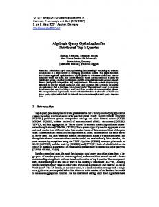
2. The 2-Way Semijoin Figure 2 The 2-way semijoin [7] evolved from the semijoin. The authors make assumptions common to most papers in the area: It is assumed that attributed values are distributed uniformly and that attributes are independent of one another. This may not be realistic but simplifies the problem. A semijoin works as follows: We assume we have two relations R1 and R2, at different sites which must be joined and they have at least one common joining attribute, j. Rij, is the projection of the relation Ri over the joining attribute j. To execute the semijoin we first form the projections d1j and d2j. The smallest projection, say d1j, is shipped to the site of R2 where a join is performed between the projection and the relation. This join eliminates tuples from R2 that would not take part in a join of the two relations. Thus, R2 is reduced. The amount of reduction depends on the number of common values in the joining attribute: The more in common, the greater the reduction. This is known as the selectivity of the reducing relation and we will define it formally later in the paper. To show how the semijoin works we use the following simple example: Given two relations R1 and R2 that are at different sites: R1

S#

Sname

2

R2

S#

Rank

Ahmed

2

100

3

Smith

4

5

Chen

6 8

In a 2-way semijoin [7], the first step is exactly as in a semijoin. The projection d1j is sent to the site of R2. Then the tuples in R2 are divided into two distinct groups: Those where the S# matches the S# from R1 (M) and those where the S# values do not match (NM). In this case M and NM are: M

S#

NM

2

2

6

4

8

10 12 Figure 3

Now, the smaller of M and NM is sent back to R1 to reduce it. In this example, M, would be sent back and R1' would be reduced to: R1'

S#

Sname

200

2

Ahmed

6

100

6

Saha

Saha

8

100

8

Jones

Jones

10

200

12

300

Figure 1 We project R1 over S# and transmit the values to the site of R2 and perform a join there. Thus R2 will be reduced to R2', as shown in figure 2:

S#

Figure 4 Both R1' and R2' are now sent to the query site for the final join. In [7] the authors conclude that 1.

The 2-way semijoin works better than a single semijoin.

2.

Using a 2-way semijoin will greatly improve the reduction power of the reduced relations.

No actual method for incorporating the 2-way semijoin into an algorithm is given in [7]. It is suggested as future work. An algorithm is later proposed in [8] but it is quite

basic. The emphasis of the paper [8] is not so much about developing an algorithm but, rather, the stress is placed on making the algorithm efficient through the use of a pipeline n-way planner. The authors also propose, as future work, integrating 2-way semijoins into existing semijoin algorithms by either replacing all semijoins by either 2-way semijoins or a combination of semijoins and 2-way semijoins. We are not aware of any work done on this proposal. It is clear, except in anomalous cases, that the 2-way semi-join will always outperform a single semijoin as it reduces two relations, not one. In this paper we investigate how the 2-way semijoin compares to two single semijoins. In our opinion, this appears to be a more informative comparison.

3. Our Work Our objective is to experimentally compare the performance of the 2-way semijoin [7] with an algorithm where we simply perform two separate semijoins between two relations. In our semijoins we deliberately do not distinguish between matching (M) and non-matching (NM) tuples, so that we can investigate its effects and usefulness. 3.1 Definitions For our algorithm to work, we need certain information [14]. For each relation we know ⎮Ri⎮, the number of tuples in the relation and S(Ri), the size of the relation in bytes. For each projection, dij, we know the cardinality of dij, ⎮dij⎮and its size in bytes, S(dij). We know the cardinality of the domain for each dij, denoted by ⎮D(dij)⎮. That is, the number of values that may possibly occur as opposed to the actual values that appear in the projection. We know the selectivity of each joining attribute. The selectivity is formally defined as [14]: ρ = ⎮ dij⎮/⎮D(dij)⎮ The selectivity values range from 0 to 1. Informally, the selectivity of an attribute is referred to as its reduction power. That is, the amount of reduction depends on the selectivity of the reducing relation. Counter intuitively, the closer the value is to zero, the greater the selectivity of the projection and its reduction power on other relations. With each semijoin (), there is an associated cost, benefit and profit [14]. The cost of a semijoin is defined as: C(dij  dkj ) = C0 + S(dij) × C1 where C0 is the start up cost associated with the transmission of data and C1 is a constant cost related to data transmission. In our work, we assume that C0 is zero and C1 is one. This does not affect our findings as we

applied the same assumption to our execution of the 2-way semijoin. This is also assumed in other papers. The benefit of a semijoin is defined as: B(dij  dkj) = S(Rk) − (S(Rk) × ρ (dij)) Profit is the difference between the cost and the benefit of the semijoin: P(dij  dkj ) = B(dij  dkj ) − C(dij  dkj ) We only execute profitable semijoins. That is, where P(dij  dkj ) > 0. 3.2 Our Algorithm and Experiments We performed our experiments using a simulator program. This program built and populated the relations for the execution of both the 2-way semijoin and the two separate semijoins. We worked with two different relations at a time for both methods. We had one designated joining attribute. In each relation we varied the number of attributes, from 3 to 7; the number of bytes in each attribute, from 30 to 500; the number of tuples in the relation, from 100 to 2000; the domain sizes, from 500 to 4000 and the selectivity. The selectivity was varied very precisely so that we covered, in sequence, most possible values. However, we decided to examine 3 specific bands of values. Namely, high, medium and low: 0 . ρ -0.33, 0.34 . ρ -0.66 and 0.67 . ρ - 1 The relations were populated using the domains of the attributes in each relation. We used a random number generator to chose the values. One common attribute was chosen for joining the two relations. We assumed that the two relations were at different sites. Also, we assumed that the cost to transfer an attribute value from one site to another was its size in bytes. Thus, to transfer 5 bytes, the cost is 5 units. In keeping with [7] our goal was to minimize the amount of data transferred between the two sites of the relations. Our program ensured that each query was correct in the sense that, for example, the projection size and the selectivity were properly related and made sense. It executed both methods recording the cost, benefit and profit for each of 1000 random queries in each selectivity band. After the values were recorded we calculated the average cost, benefit, profit and improvement. From this we got the results shown in Table 3. There are three basic steps to our algorithm: 1. First, we generate and populate the two relations for the 2-way semijoin and our two separate semijoins. 2.

We perform a 2-way semijoin [7] on the relations, recording the cost, benefit and profit.

3.

We perform two separate semijoins, using the same relations, recording the cost, benefit and profit. However, as previously stated, we do not distinguish between matching and non-matching tuples.

Thus, for each query, we first performed a 2-way semijoin as outlined in [7] and then we performed two separate semijoins, using the same two relations in each case. We varied the sizes of the relation, attributes and number of attributes in each query. We recorded all data required for our analysis and results. In keeping with the 2-way semijoin [7], there were only two relations in each query and one common joining attribute. 3.3 Some worked examples These are not actual cases from our experiments but are simplified examples to illustrate our methodology. The assumptions made about the relative sizes of M and NM are, however, based on what we saw in our experiments. In these examples ⎮D(dij)⎮ = 1000 for every attribute. Example 1: High selectivity band R R1 R2

S(Ri) 1000 2000

⎮dij⎮

ρ⎮dij⎮

200 300

0.2 0.3

Table 1 We first perform two separate semijoins. With R1  R2 the cost is 200, the size of the projection. ⎮R2'⎮ = 2000 × 0.2 = 400, so the benefit is 1600 and the profit is 1400. Next we perform the second semijoin using the reduced R2'. For R2'  R1 the cost is 300. The benefit is 1000 – 300 = 700. The profit is 400. The total profit for our method is 1400 + 400 = 1800. Note: We cannot estimate the reduction in the size of the projection so it is common practise in the literature to assume it is not reduced although this will not be the case. We follow common practise here in our examples. However, in our experiments we know exactly the size of the reduction. Next we execute the 2-way semijoin. However, in this case we assume, given the high selectivity, that NM is much smaller than M so we set NM to 150, based on observations from our test cases. The first part of the 2-way semijoin is exactly the same as in our method. So, with R1  R2, the cost is 200, the benefit is 1600 and the profit is 1400. However, the backward semijoin is different because the NM set of values is sent back. Now the cost is 150. ⎮R1'⎮ = 1000 × 0.3 = 300, so the benefit is 700 and the profit is 550. The total profit for the 2-way semijoin method is 1400 + 550 = 1950.

We calculate the percentage improvement as follows: The difference in total profit is 1950 − 1800 = 150. Then our result is (150/1800) × 100, an 8.3% improvement by the 2-way semijoin over our method.

Example 2: Middle selectivity band R R1 R2

S(Ri) 4000 5000

⎮dij⎮

ρ⎮dij⎮

500 550

0.5 0.55

Table 2 Again, we first perform two separate semijoins. For R1  R2, the cost is 500. ⎮ R2'⎮ = 5000 × 0.5 = 2500. Therefore, the benefit is 2500 and the profit is 2000. Now we perform the next semijoin using the reduced R2'. For R2'  R1 the cost is 550. ⎮R1'⎮ is 2200, the benefit is 1800 and the profit is 1250. In this example, the total profit for our method is 2500+1250 = 3250. Next we execute the 2-way semijoin. However, in this case we assume, given the selectivity is almost right in the middle, that M is very slightly smaller than NM so we set M to 500. For R1  R2, the cost is 500, the benefit is 2500 and the profit is 2000. For the backward semijoin the cost is 500. ⎮R1'⎮ = 4000 × 0.55 = 2200, so the benefit is 1800 and the profit is 1300. The total profit for the 2-way semijoin method is 2000 + 1300 = 3300. The final calculation is (50/3300) × 100, a 1.5% improvement. In this example the improvement is very small. We conclude that this happened because there was very little difference in the selectivity values and they were almost right in the middle of the range. This may explain why we only get a 2.5% difference between two separate semijoins and the 2-way semijoin in this middle band in our experiments. Most selectivity values are close to the middle but at the boundaries the difference between M and NM is somewhat greater and will give a bigger difference in performance. When the selectivity values get very low, for example 0.9, the semijoin most likely would not be profitable. We did not perform unprofitable semijoins but they did occur in our experiments when the selectivity values were very low. It is not clear what was done in [7] and [8].

4. Our Results In all cases, on average, the 2-way semijoin outperformed the execution of two separate semijoins. The 2-way semijoin performed significantly better in the higher and lower selectivity bands.

The following table summarizes our results:

Selectivity 2-way average total profit 2 semijoins average total profit Improvement

High

Middle

Low

4995

6742

3263

4437

6573

2979

9.4%

2.5%

8.7%

Table 3 With high selectivity the difference in performance was 9.4%; with low selectivity the difference was 8.7%. In both cases this is a significant difference. We conclude that the disparity is so big because in the 2-way semijoin the smaller of M or NM is returned in the backward phase of the semijoin. This will always be much smaller than sending back the entire projection as we did in our two separate semijoins. Clearly, making the division between M and NM is very advantageous in this case. However, in the middle selectivity band the difference was only 2.5%. This can be explained by noting that in this case the difference between M and NM will be small and thus the amount of data returned by both methods will be very similar. However, the difference will be bigger at the boundaries of the band and hence the 2-way semijoin still performs better than our method. Our results make sense because when there is a large difference between M (matching) and NM (non-matching) attribute values, as happens in the higher and lower selectivity bands, sending the smaller of N or MN will significantly reduce the amount of data sent in the backward phase of the 2-way semijoin. However, when there is not much difference between N and NM then the advantage of sorting the tuples is diminished. Thus, in these cases two separate semijoins will be approximately as profitable as the 2-way semijoin without the overhead of dividing the tuples into two different sets. Note that in our two separate semijoins, the set M is always returned to the reducing relation. This is common practice in algorithms employing semijoins. As there is an overhead associated with the division of tuples into N and NM, albeit relatively small, we recommend the following: When the selectivity is in the higher or lower band, then use the 2-way semijoin. If the selectivity is in the middle band, then use two separate semijoins as there is slightly less overhead and the results produced are exactly the same.

5. Conclusion In our work we conclude that the 2-way semijoin should be used when the selectivity of the reducing attribute is

either high or low. If the selectivity is in the middle range then two separate semijoins will produce the same final result and will perform almost as well without the overhead of dividing the reduced attribute values into the M and NM sets. Therefore we recommend using two separate semijoins when the selectivity is in the middle band. Whether we use a 2-way semijoin or 2 separate semijoins, the end result is the same: The reduced relations are identical. Thus we make the following conclusions, similar to those of [7]: 1.

Assume we have two relations, R1 and R2 at different sites. If R1' is produced as the result of a previous semijoin on R1 then the propagation of its reduction power is increased. That is, if R1' is used to reduce another relation then the reduction produced is greater than if R1 was used. Hence, P(R1'  R2) > P(R1  R2) Using R1', that has already been reduced, will clearly reduce R2 further than using the unreduced R1. Conversely, we will have P(R1  R2) < P(R1'  R2)

2.

Assume we have three relations R1, R2, and R3 at different sites. Again, R1' is produced by a previous semijoin. Now, if R1' is used in a strategy to reduce the other relations the reduction power is propagated and is greater. That is, P(R1'  R2  R3) > P(R1  R2  R3) In (R1  R2  R3) an unreduced R1 is used in the semijoin sequence, so there is no reduction benefit from a previous semijoin on R1. However, in (R1'  R2  R3), R1 has been reduced so it has a larger reduction effect on R2 and, subsequently, an even greater reduction power on R3. As above, the converse is true.

3.

Using an unreduced relation, say R3, to reduce R1' will be less profitable than using it to reduce the original R1. That is, P(R3  R1') < P(R3  R1) In (R3  R1) we are performing a simple semijoin on an unreduced R1. However, in (R3  R1'), R1 has already been reduced so the reduction effect of R3 is less.

4.

Performing two semijoins, by doing a forward and backward reduction, is always going to be more profitable than a single semijoin. That is, P(R1  R2  R1) > P(R1  R2) This is because (R1  R2  R1) reduces two relations while (R1  R2) will only reduce one. This is similar to a stated premise and contribution of [7]. However, we considered this comparison to be inequitable. Hence, we performed what we considered to be a more informative comparison: Namely, evaluate the

2-way-semjoin with two separate semijoins to see what the effects would be. Our work has some limitations: 1.

2.

3.

4.

We performed an experimental rather than analytical comparison of the two methods. We did this because no algorithm was suggested in [7] and the algorithm proposed in [8] was not considered suitable. However, we recognize that experiments can be flawed, especially if the data is skewed in some unintended way. More thought should have been put into the design of our experiments. We recognize that there are some flaws. However, intuitively, our conclusions seem correct. In future work we would design a better experimental platform that examines a larger number of parameters and varies them in a more predicable way. This might lead to a more significant contribution to the research area. It would also validate our results in this work. We did not perform a time and space complexity analysis of the cost of dividing the joining attribute values into M and NM. We didn’t do so since we concluded, from the results of our experiments, that the benefit far outweighs the overhead cost when the selectivity is high or low. We can make no definitive statement about the middle selectivity band but still believe, in this case, that the cost of the division is very close to that done in traditional semijoins and therefore should make very little difference. We did not apply any statistical testing to our results. Future work would entail applying a standard test should as the TPC benchmark to give more validity to our results.

As a possible application, we are currently in the process of developing a semijoin based algorithm where we compare using a mixture of semijoins and 2-way semijoins with using semijoins entirely. In contrast to the conclusions made in [7], our initial results are not producing significantly different results. It is clear that we need to develop a better algorithm as 2-way semijoins are undoubtedly very beneficial.

Acknowledgements We wish to thank the reviewers for their very helpful comments. This research was fully funded by a research grant from NSERC to Joan Morrissey.

References [1] J.K. Ahn, & S.C. Moon, Optimizing joins between two fragmented relations on a broadcast local network. Info. Syst., 16(2), 1991, 185-198. [2] P. Legato, P.G. Paletta, & L. Palopoli, Optimization of join strategies in distributed databases. Info. Syst., 16(4) 1991, 363-374. [3] P.A. Bernstein, N. Goodman, E. Wong, C.L. Reeve, & J. Rothnie, Query processing in a system for distributed databases (SDD-1). ACM Trans. on Database Systems, 6(4), 105-128, 1981. [4] P.A. Black, & W.S. Luk, A new heuristic for generating semi-join programs for distributed query processing. Proc. IEEE COMPSAC, 1982, 581-588. [5] P. Apers, A.R. Hevner, & S.B. Yao, Optimization algorithms for distributed queries. IEEE Transactions on Software Engineering, 9(1), 1983, 51-60. [6] L. Chen, & V. Li, Improvement algorithms for semijoin query processing programs in distributed database systems. IEEE Transations on Computers, 33(11 ), 1984, 959-967. [7] H. Kang, & N. Roussopoulos, Using 2-way semi-joins in distributed query processing. Proc. 3rd Int. Conf. on Data Engineering, Los Angeles, California, 1987, 644650. [8] N. Roussopoulos, & H. Kang, A pipeline N-way join algorithm based on the 2-way semi-join program. IEEE Trans. on Knowledge and Data Engineering, 3(4), 1991, 486-495. [9] L. Chen, & V. Li, Domain-specific semi-join: a new operation for distributed query processing. Info. Sci., 52(2), 1990, 165-183. [10] C. Wang, V. Li, & A. Chen, Distributed query optimization by one-shot fixed precision semi-join execution. Proc. 7th Int. Conf. on Data Engineering, Kobe, Japan, 1991, 756-763. [11] M. Chen, & P. S. Yu, Combining join and semi-join operations for distributed query processing. IEEE Transactions on Knowledge and Data Engineering, 5(3), 1993, 534-542. [12] D.M. Chiu, P.A. Bernstein, & Y.C. Ho, Optimizing chain queries in a distributed database system. Siam Journal Of Computing, 13(1), 1984, 116-134.

[13] D.M. Chiu, & Y.C. Ho, A method for interpreting tree queries into optimal semijoin expressions. ACM SIGMOD, Santa Monica, California, 1980, 169-178.

[26] G. Graefe, & K. Ward, Dynamic query evaluation plans. Proc. of ACM SIGMOD, Portland, Oregon, 1989, 358-366.

[14] J.M. Morrissey, & W.T. Bealor, Minimizing data transfers in distributed query processing: a comparative study and evaluation. The Computer Journal, 39(8), 1996, 676-687.

[27] G. Graefe, Query evaluation techniques for large databases. ACM computing surveys, 25(1) 1993, 73-170.

[15] Yue (Amber) Zhang, Variation of Bloom filters in distributed query processing. Master’s Thesis, University of Windsor, 2003. [16] J.C.R. Tseng, & A.L.P. Chen, Improving distributed query processing by hash-semijoins. Journal of Information Science and Engineering, 8, 1992.

[28] C. Mohan, D. Haderle, Y. Wang, & M. Cheng, Single table access using multiple indexes: optimization, execution and concurrency control techniques, Lecture Notes in Computer Science, Springer-Verlag, 416, 1990, 29-43. [29] D.G. Severance, & G.M. Lohman, Differential files: their application to the maintenance of large databases. ACM Transactions on database systems 11(3) 1976, 257267.

[17] B.H. Bloom, Space/time tradeoffs in hash coding with allowable errors. Comm. ACM, 13(7), 1970, 422426.

[30] J.K. Mullin, A second look at bloom filters. Comm. ACM, 26(8), 1983, 570-571.

[18] Z. Li, & K.A. Ross, PERF join: an alternative to twoway semijoin and Bloomjoin. Proc. Of CIKM, 1995, 137144.

[31] J.K. Mullin, Optimal semijoins for distributed database systems. IEEE Trans. on Software Engineering, 16(5), 1990, 558-560.

[19] A.R. Hevner, The optimization of query processing in distributed database systems. PhD thesis, Perdue University, 1980.

[32] P. Boderick, J. Pyra, & J.S. Riordan, Correcting execution of distributed queries. Proc. of 2nd Int. Symp. on Databases in Parallel and Distributed Systems, Dublin, Ireland, 1990, 192-201.

[20] A. L. Chen, & V. Li, Domain specific semijoin: a new operation for distributed query processing. Information Sciences, 52(2) , 1990, 165–183.

[33] P. Boderick, J.S. Riordan, & J. Pyra, Deciding to correct distributed query processing. IEEE Trans. on Knowledge and Data Engineering, 4(3), 1992, 253-265.

[21] D.J. DeWitt, S. Ghandeharizadeh, D. Schneider, A. Bricker, H. Hsiao, & R. Rasmussen, The GAMMA database machine project. IEEE Transactions on Knowledge and data engineering, 1990, 44-62.

[34] W. Perrizo, & C. Chen, Composite semijoins in distributed query processing. Information Science, 50(2), 1990, 197-218.

[22] G.Z. Qadah, Filter-based join algorithms on uniprocessor and distributed-memory multiprocessor database machines, Lecture Notes in Computer Science, Springer Verlag, 303, 1988, 388-413.

[35] P. Boderick, J.S. Riordan, & C. Jacob, Dynamic distributed query processing techniques. Proc. 17th Annual ACM Computer Science conference, Dallas, Texas, 1989, 348-357.

[23] G.Z. Qadah, & K.B. Irani, The join algorithms on a shared-memory multiprocessor database machine. IEEE Transactions on Software Engineering, 1988, 1168-1683. [24] P. Valduriez, & G. Gardarin, Join and semijoin algorithms for a multiprocessor database machine. ACM Transactions on Database Systems 9(1), 1984, 133-161. [25] J.K. Mullin, Estimating the size of a relational join. Information Systems, 18(3), 1993, 189-196.