KSCE Journal of Civil Engineering (2016) 20(1):478-484 Copyright ⓒ2016 Korean Society of Civil Engineers DOI 10.1007/s12205-015-1282-3
Water Engineering
pISSN 1226-7988, eISSN 1976-3808 www.springer.com/12205
TECHNICAL NOTE
Investigation Internal Parameters of Neural Network Model for Flood Forecasting at Upper River Ping, Chiang Mai Tawee Chaipimonplin* Received May 17, 2013/Revised December 29, 2014/Accepted December 30, 2014/Published Online January 31, 2015
··································································································································································································································
Abstract The flood issue for forecasters at Chiang Mai derives from the monsoon rainfall, which leads to serious out-of-bank flooding two to four times a year. Data for stage and rainfall per hour in Upper Ping catchment is limited as the historical flood record is limited in length. Neural Network forecasting models are potentially very powerful forecasters where the data are limited. However, insufficient data for Neural Network training reduces the model performance. All data for Neural Network is divided into three datasets: training, validation and testing. In addition most of learning algorithms require validation data unlike Bayesian Regularization (BR) algorithm with no validation data. The power of BR to forecast effectively where data set are limited. Therefore, this algorithm is worth exploring for the Upper Ping catchment, also comparison performance with the Levenberg-Marquardt algorithm (LM) that is the fastest training. In addition, for the best model performance hidden nodes are set as 50%, 75% and 2n+1 of input nodes. The Neural Network model is used to predict water stage at P.1 and P.67 station at lead times of 6 and 12 hours with two different learning algorithms. The results have found that Neural Network performance training with LM algorithm is better than BR algorithms by improving the peak stage. The overall performance of the model that has the hidden nodes less than input nodes of 50% and 75% has the best performance. Keywords: neural network, flood forecasting, bayesian regularization, levenberg-marquardt, internal parameters, upper river ping, chiang mai ··································································································································································································································
1. Introduction Monsoon rainfall leads to serious flooding in Thailand almost every year. Particularly in 2011, the tropical storm NOCK-TEN hit Thailand and caused flood over northern, upper northeastern and central part of Thailand were affected by flood and 46 death (Department of Disaster Prevention and Mitigation, 2011). There are many types of flood modeling such as physical based model or conceptual model or black box model. The disadvantage of physical and conceptual model is it required many physical data. In contrast, neural network is one of the black box models and does not need lots of physical data. The big advantage of neural network is the ability to generalize the unseen data and does not concern the physical relationships. The use of neural networks can be found throughout different areas of hydrology and water resource management. The ASCE review into the use of neural networks in hydrology considered applications across a range of areas including rainfall-runoff modeling, modeling streamflows, water quality modeling, ground water applications, estimation of precipitation and miscellaneous areas such as reservoir operation and flood wave propagation (ASCE, 2000a). The Upper River Ping, which is study area, is a large catchment with very limited long-term data records. Calibrating a physical
or conceptual model for a catchment of this size is inherently very difficult; many parameters would have to be estimated rather than known quantities within such a model. There are limited data available for hour stage at stations on the River Ping that can be used to drive a neural network model. The city of Chang Mai in the lower part of the catchment is at risk to flooding, and would benefit from effective real-time flood warning. The black box neural network model approach offers the opportunity to create models that can be run in real-time, and which can be updated relatively easily as new data become available each year. In order to improve the neural network model performance, internal parameters are the key. There are many internal parameters of neural network model i.e. learning algorithms, number of hidden layers, number of hidden nodes, learning rates, momentum rates, ranges of normalization, transfer function (Maier and Dandy, 1998). There have been many investigations internal parameters for model improvement such as to compare the performance of different learning algorithms (Fun and Hagan, 1996; Piotrowski and Napiorkowski, 2011; Yonaba et al., 2010), or to determine the number of hidden node (Chen et al., 2010; Dawson and Wilby, 1999; Lorrai and Sechi, 1995; Sattari et al., 2012; Wang et al., 2009; Yoon et al., 2011) or to explore
*Lecturer, Faculty of Social Sciences, Dept. of Geography, Chiang Mai University, 50200, Thailand (Corresponding Author, E-mail:
[email protected]) − 478 −
Investigation Internal Parameters of Neural Network Model for Flood Forecasting at Upper River Ping, Chiang Mai
difference of normalization ranges (Derakhshan and Talebbeydokhti, 2011; Varoonchotikul, 2003), or to investigate on transfer function types Yonaba et al., 2010; Varoonchotikul, 2003), or to use several momentum rates (Yoon et al., 2011), or to apply the variety of learning rates (Yoon et al., 2011; Derakhshan and Talebbeydokhti, 2011; Maier and Dandy, 1996) or to compare between one and two hidden layers (Lorrai and Sechi, 1995; Derakhshan and Talebbeydokhti, 2011; Maier and Dandy, 1996). However, all papers could not strongly conclude which internal parameters are the best choices for the best performance due to the uncertain of data driven in the study area. ASCE suggested that for the best setting internal parameters in the neural network model for each study area, trial and error is necessary (ASCE, 2000b). Therefore, this paper investigates the learning algorithms and number of hidden nodes that suitable for the best model performance in the Upper River Ping for flood forecasting at P.1 and P.67 station.
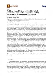
2. Study and Data The Ping catchment is in northern part of Thailand. The area of entire catchment is 33,898 km2 and with average annual rainfall between 900-1,900 mm. The river Ping is the main river in this catchment that reaches up to 740 km long (Fig. 1). The Ping catchment can be divided into two parts; Upper and Lower Ping and the study area for this paper is located in the Upper Ping catchment. There are several water stage stations in the study area such as P.1 (located in the Chiang Mai city), P.67 or P.75 (located near to Dam) (Fig. 2). The current technique for
Fig. 2. Study Area (Hydrology and Water Management Centre for Upper Northern Region, 2007)
flood warning in Chiang Mai city is based on the correlation between water stage P.67 station and P.1 station and the warning time is approximately 6-7 hr (Hydrology and Water Management Centre for Upper Northern Region, 2012). As the data limited of the hourly rainfall in this catchment, then the radar images are used as the rainfall data. The radar image is operated by the bureau of Royal Rainmaking and Agriculture Aviation. The radar is the CAPPI radar (Constant Altitude Plan Position Indicator) that uses to detect precipitation with a ground coverage radius of 240 km (Fig. 3). The related paper that used this radar image for flood forecasting at P.1 station can be found in Chaipimonplin et al. (2010). However, in this paper the radar image was used for flood forecasting at P.67 station that is located above P.1 station and six sample points are selected over the study area (Fig. 4). The dataset that was available on both water stage and radar image is in year 2005 and only data from the monsoon season were then used to develop and test the neural network models. The first storm was used for testing because it contains the
Fig. 1. Ping Catchment (Department of Water Resources, 2007) Vol. 20, No. 1 / January 2016
− 479 −
Fig. 3. Sample of Radar Image
Tawee Chaipimonplin
3. Methodology and Performance Measures
algorithm (MathWorks, 2012a). Bayesian Regularization (BR) algorithm is the function of neural network for training by updating the weight and bias values that according to LM optimization. BR algorithm reduces a combination of squared errors and weights and determines the correct combination (MathWorks, 2012b). Two papers (Fun and Hagan, 1996; Piotrowski and Napiorkowski, 2011) compared the performance of different algorithms and found that LM produced the best performing result. BR is another type of training procedure that can be applied to LM (Foresee and Hagan, 1997; Mackay, 1992) and essentially reduces the impact of the network weights. It simultaneously minimizes the overall error function and the sum of the squared weights. A big advantage of the BR algorithm is that it does not require a validation data set and therefore makes BR a potentially suitable algorithm where data are limited (Beale et al., 2011). This means that more data are available for the training process. The BR algorithm has been used in a few hydrological modeling applications (Chaipimonplin et al., 2010; 2011a Anctil and Lauzon, 2004; Anctil et al., 2006; Anctil et al., 2004; Zhang and Govindaraju, 2000; Napolitano et al., 2010). To compare the most common used and fast Learning algorithm (LM) with algorithm for limited data (BR) thus the neural network models are trained with LM and BR in the Matlab 2011a. Both BR and LM algorithm were run 50 times, taking the average of the 50 runs as the model forecast (after Anctil and Lauzon, 2004). The models were designed to forecast water stage lead time at 6 and 12 hour. Model A has 7 input variables; 5 water stages, which is the station for stream flow (P.1t, P.67t, P.67t-6, P75t and P75t-6) and 2 outflows (flow t and moving average t-6) and forecast water stage at P.1 station. Model B has 14 input variables; 12 radars (Z11t, Z11t-6, Z12t, Z12t-6, …, Z23t-6) and 2 water stages (P75t and P75t-6) and forecast water stage at P.67 station.
3.1 Learning Algorithms There are many types of backpropagation algorithm, which can be classified into two main groups. The first group is described as slow learning and uses batch gradient descent or simple gradient descent with momentum. The second, fast learning, group may employ Conjugate Gradient Descent (CGD), QuasiNewtonian (QN) algorithms (which require more storage and computation for each iteration) and the Levenberg-Marquardt (LM) numerical optimization technique. The fast learning techniques can perform 10 to 100 times the speed of the slow learning processes. The difference between CGD and simple gradient descent is that it does not proceed along the direction of the error gradient but in a direction orthogonal to the one in the previous time step. The advantage for the modeler is a relatively fast training time. It has been used in hydrology for short and longer term stream flow forecasts (Kisi, 2007). LM algorithm is probably the most commonly employed algorithm (Beale et al., 2011) and is strongly recommended as a first choice supervised
3.2 Hidden Nodes The most common neural network arrangement is three layers: the input layer, where data are supplied to the model, a hidden layer, necessary for processing, and an output layer, where the forecast or prediction is produced. In addition there are bias nodes necessary for the calculations to work. The number of hidden layers and hidden layer nodes is determined by the operator. Some neural networks have more than one hidden layer although it has been shown that any continuous function can be approximated with this neural network structure using only one hidden layer (Hornik, 1993). Where the model has a very large number of hidden layer nodes, this process can be very efficient. However, where the input nodes and weights are small, there does not appear to be any advantage in using CGD over first order backpropagation methods. The number 1, 2 and 3 which indicated the percentage of hidden nodes, 2n+1, 75% and 50% of input nodes, respectively (Table 1).
Fig. 4. Sample Points
Fig. 5. All Five Storms, Year 2005
biggest event on record then the training dataset selected four storms (September to November) (Fig. 5).
− 480 −
KSCE Journal of Civil Engineering
Investigation Internal Parameters of Neural Network Model for Flood Forecasting at Upper River Ping, Chiang Mai
Table 1. Model Architectures Model A1 A2 A3 B1 B2 B3
Table 2. Performance of Models at P.1 Station
Architecture 7:15:1 7:5:1 7:3:1 14:29:1 14:11:1 14:7:1
Model T+6 LM_A1 LM_A2 LM_A3 BR_A1 BR_A2 BR_A3
3.3 Performance Measures To compare the models performance, Root Mean Square Error (RMSE) and Coefficient of Efficiency (CE) are used to evaluate the model performance (Dawson et al., 2007). The RMSE is written as: 2 1 n RMSE = --- Σi = 1 ( Li – Lˆ i ) n
(1)
Model T+12 LM_A1 LM_A2 LM_A3 BR_A1 BR_A2 BR_A3
RMSE Train 0.023 0.043 0.052 0.018 0.037 0.049
CE Test 0.123 0.101 0.119 0.209 0.132 0.154
Train 0.999 0.997 0.996 0.999 0.998 0.996
Test 0.357 0.246 0.222 0.430 0.301 0.324
Train 0.998 0.992 0.987 0.999 0.994 0.988
RMSE Train 0.035 0.076 0.097 0.027 0.065 0.091
Test 0.986 0.991 0.987 0.961 0.984 0.979 CE
where, n is the number of forecasts, Li and Lˆ i are the observed and forecasted water stage at time i, respectively. The RMSE value is close to 0, it means the model performance for forecasting water stage is perfect. The CE is written as: 2 n Σ i = 1 ( Li – Lˆ i ) CE = 1− ----------------------------(2) 2 n Σi = 1 ( Li – L ) where, L is the average of observed water stage. When the CE value is close to 1, it means the model performance of forecasting water stage is perfect.
4. Results 4.1. Result at P.1 Station Figure 6 contains the plots of actual and predicted stage for four storms in 2005 with x axis is time (day/month/year) and y axis is water stage (meter). The overall training performances of all models are good learning as the predicted stage similar with actual stage. The statics reveal that the model BR_A1 is the best model for training both t+6 and 12 hr but model LM_A2 is the best for testing (Table 2). In addition, these results clearly show that when decreasing the number of hidden nodes the error of training model (RMSE value) increases or the accuracy decreases (CE value). In contrast, model trained with LM and hidden nodes less than input nodes is the best for forecasting water stage at P.1 station. For further analysis of the models performance, Fig. 7 presents the hydrographs of t+6 and 12 hr at P.1 station. Those models LM performances are slightly better than BR models, particularly at the peak stage as model LM_A2 (hidden node 75% of input nodes) predicted very close to actual stage at t+6 hr and model LM_A3, which has hidden node 50% of input nodes, is the best model for forecasting water stage at t+12 hr. Vol. 20, No. 1 / January 2016
− 481 −
Fig. 6. Training Hydrographs of Model A
Fig. 7. Testing Hydrographs of Model A
Test 0.886 0.946 0.956 0.834 0.919 0.906
Tawee Chaipimonplin
Fig. 8. Training Hydrographs of Model B
Fig. 9. Testing Hydrographs of Model B
4.2 Result at P.67 Station The results of training models are shown in Fig. 8, the overall training performances of all models are good performance but not good as training at P.1 station. Statics of the all models are summarized in Table 3. These results clearly show that the overall performance of the training with BR algorithm is better than LM as the RMSE and CE are all better, also the RMSE value increases when decrease number of hidden nodes (same as P.1 station). For forecasting water stage at P.67, model LM_B2, which has hidden nodes 75% of input node, is the best model for t+6 hr as CE value is the highest and RMSE value is the lowest. Also model LM_B3, which has hidden node 50% of input nodes, is the best model for forecasting water stage at t+12 hr. Figure 9 is the hydrograph of testing models at t+6 and 12 hr, it is obvious that all models LM predicted good performance parti-
cularly at the peak stage, while all models of BR predicted bad performance at the peak stage. The model B performance both training with LM and BR are different when compare with model A as model LM_B has better performance than model BR_B (Fig. 9) unlike model LM_A and BR_A that have similar results (Fig. 7). It could be explained that input variables for model A are hydrology data (water stage and outflow) but for model B use hydrology and radar data (water stage and radar image). As a result, the different types of input variable could influence the learning performance of BR algorithm.
Table 3. Performance of Models at P.67 Station Model T+6 LM_B1 LM_B2 LM_B3 BR_B1 BR_B2 BR_B3 Model T+12 LM_B1 LM_B2 LM_B3 BR_B1 BR_B2 BR_B3
RMSE Train 0.141 0.151 0.167 0.126 0.134 0.160
CE Test 0.410 0.386 0.400 1.099 0.810 0.474
Train 0.982 0.979 0.975 0.986 0.984 0.977
Test 0.305 0.326 0.277 0.895 0.605 0.575
Train 0.981 0.977 0.971 0.986 0.982 0.972
RMSE Train 0.146 0.159 0.180 0.124 0.141 0.176
Test 0.920 0.929 0.923 0.422 0.686 0.893 CE Test 0.955 0.949 0.963 0.616 0.825 0.841
5. Conclusions For forecasting water stage at t+16 and t+12 both P.1 and P.67 station, the results show that the LM algorithm clearly proved to have an overall advantage over the BR algorithm on its own in terms of forecasting accuracy, especially with the different types of input variables. It could be concluded that LM has the ability to learn more variety of input variables than BR. Moreover, model performance was improved by selecting the number of hidden nodes 50% and 75% of input nodes (LM_A2, LM_A3, LM_B2 and LM_B3) when forecasting t+12 and t+6 hr. The results can be compared to the similar research, which trained model with LM and BR for flood forecasting at P.1 station, concluded that BR is better than LM algorithm (Chaipimonplin et al., 2011b). The difference between this paper and that research are the version of Matlab software (2006b and 2011a), input variables (water stage, radar and water stage, outflow) and rang of dataset (training 2001-2004, testing 2005 and training four storms 2005, testing first storm 2005). Consequently, the further investigation on dataset for testing and training, more different learning algorithms and determination input variables would be highly recommended for the best performance in this catchment.
− 482 −
KSCE Journal of Civil Engineering
Investigation Internal Parameters of Neural Network Model for Flood Forecasting at Upper River Ping, Chiang Mai
Acknowledgements Thank you to the Hydrology and Water Management Center for the Upper Northern Region for the water stage data, also the Bureau of Royal Rainmaking and Agricultural Aviation for the radar images. This research was funded by Faculty of Social Sciences, Chiang Mai University.
References Anctil, F. and Lauzon, N. (2004). “Generalisation for neural networks through data sampling and training procedures, with applications to streamflow predictions.” Hydrology and Earth System Sciences, Vol. 8, pp. 940-958. Anctil, F., Lauzon, N., Andreassian, V., Oudin, L., and Perrin, C. (2006). “Generalisation for neural networks through data sampling and training procedures, with applications to streamflow predictions.” Journal of Hydrology, Vol. 328, Nos. 3-4, pp. 717-725. Anctil, F., Michel, F., Perrin, C., and Andreassian, V. (2004). “A soil moisture index as an auxiliary ANN input for stream flow forecasting,” Journal of Hydrology, Vol. 286, Nos. 1-4, pp. 155-167. Anctil, F., Perrin, C., and Andreassian, V. (2004). “Impact of the length of observed records on the performance of ANN and of conceptual parsimonious rainfall-runoff forecasting models.” Environmental Modeling & Software, Vol. 19, No. 4, pp. 357-368. ASCE (2000a). “Artificial neural networks in hydrology, II: Hydrologic applications.” Journal of Hydrologic Engineering, Vol. 5, No. 2, pp. 124-137. ASCE (2000b). “Artificial neural networks in hydrology, I: Hydrologic applications.” Journal of Hydrologic Engineering, Vol. 5, No. 2, pp. 115-123. Beale, M. H., Hagan, M. T., and Demuth, H. B. (2011). Neural Network Toolbox TM 7: User's guide, http://www.mathworks.com. Chaipimonplin, T., See, L. M., and Kneale, P. E. (2010). “Using radar data to extend the lead time of neural network forecasting on the River Ping.” Disaster Advances, Vol. 3, No. 3, pp. 35-43. Chaipimonplin, T., See, L. M., and Kneale, P. E. (2011a). “Improving neural network for flood forecasting using radar data on the Upper Ping river.” Proceeding 19th International Congress on Modelling and Simulation, Modelling and Simulation Society of Australia and New Zealand, pp. 1070-1076, (MODSIM2011). Chaipimonplin, T., See, L. M., and Kneale, P. E. (2011b). “Comparison of neural network learning algorithms: BR and LM, for flood forecasting, Upper Ping catchment.” Proceeding 10th International Symposium on New Technologies for Urban Safety of Mega Cities in ASIA, Chiang Mai, Thailand, (USMCA 2011) (poster). Chen, C. S., Chen, B. P. T., Chou, F. N. F., and Yang, C. C. (2010). “Development and application of a decision group back-propagation neural network for flood forecasting.” Journal of Hydrology, Vol. 385, Nos. 1-4, pp. 173-182. Dawson, C. W. and Wilby, R. (1999). “A comparison of artificial neural networks used for river flow forecasting.” Hydrology and Earth Sciences, Vol. 3, No. 4, pp. 529-540. Dawson, C. W., Abrahart, R. J., and See, L. M. (2007). “Hydro test: A web-based toolbox of evaluation metrics for the standardized assessment of hydrological forecasts.” Environmental Modelling & Software, Vol. 22, No. 7, pp. 1034-1052. Department of Disaster Prevention and Mitigation (2011). Flood Situation report, http://disaster.go.th/dpm/flood/flood.html.
Vol. 20, No. 1 / January 2016
Department of Water Resources (2007). Ping catchment, http://mekhala. dwr.go. th/mekhala/Basin_North.asp. Derakhshan, H. and Talebbeydokhti, N. (2011). “Rainfall disasggregation in non-recording gauge stations using space-time information system.” Scientia Iranica, Vol. 18, No. 5, pp. 995-1001. Foresee, F. D. and Hagan, M. T. (1997). “Gauss-Newton approximation to Bayesian learning.” Proceeding the 1997 International Joint Conference on Neural Network, pp. 1930-1935. Fun, M. H. and Hagan, M. T. (1996). Levenberg-Marquardt training for modular networks.” Proceeding the 1996 International Conference on Neural Network, Vol. 1, pp. 468-473. Hornik, K. (1993). “Some new results on neural network approximation.” Neural Networks, Vol. 6, No. 8, pp. 1069-1072. Hydrology and Water Management Centre for Upper Northern Region, (2007). Upper northern region flood warning brochures, http:// www.hydro-1.net/. Hydrology and Water Management Centre for Upper Northern Region, (2012). http://www.hydro-1.net/08HYDRO/PORTAL/IMAGES/ 100119-BOAD-P.1aaaa.jpg. Kisi, O. (2007). “Streamflow forecasting using different artificial neural network algorithms.” Journal of Hydrologic Engineering, Vol. 12, No. 5, pp. 532-539. Lorrai, M. and Sechi, G. M. (1995). “Neural net for modeling rainfallrunoff transformations.” Water Resources Management, Vol. 9, pp. 299-313. Mackay, D. J. C. (1992). “Bayesian interpolation.” Neural Computation, Vol. 4, No. 3, pp. 415-447. Maier, R. H. and Dandy, G. C. (1996). “The use of artificial neural networks for the prediction of water quality parameters.” Water Resources Research, Vol. 32, No. 4, pp. 1013-1022. Maier, R. H. and Dandy, G. C. (1998). “The effect of internal parameters and geometry on the performance of back-propagation neural network: An empirical study.” Environmental Modelling & Software, Vol. 13, No. 2, pp. 193-209. MathWorks (2012a). Documentation-Neural Network Toolbox, http:// www.mathworks.com/help/toolbox/nnet/ref/trainlm.html. MathWorks (2012b). Documentation-Neural Network Toolbox, http:// www.mathworks.com/help/toolbox/nnet/ref/trainbr.html. Napolitano, G., See, L., Calvo, B., Savi, F., and Heppenstall, A. (2010). “A conceptual and neural network model for real-time flood forecasting of the Tiber River in Rome.” Physics and Chemistry of the Earth, Vol. 35, Nos. 3-5, pp. 187-194. Piotrowski, A. P. and Napiorkowski, J. J. (2011). “Optimizing neural network for river flow forecasting-Evolutionary computation methods versus the Levenberg-Marquardt approach.” Journal of Hydrology, Vol. 407, Nos. 1-4, pp. 12-27. Sattari, M. T., Yurekli, K., and Pal, M. (2012). “Performance evaluation of artificial neural network approaches in forecasting reservoir inflow.” Applied Mathematical Modelling, Vol. 36, No. 6, pp. 26492657. Varoonchotikul, P. (2003). Flood forecasting using artificial neural networks, A.A Balkema, Lisse, The Netherlands. Wang, W. C., Chau, K. W., Cheng, C. T., and Qiu, L. (2009). “A comparison of performance of several artificial intelligence methods for forecasting monthly discharge time series.” Journal of Hydrology, Vol. 374, Nos. 3-4, pp. 294-306. Yonaba, H., Anctil, F., and Fortin, V. (2010). “Comparing sigmoid transfer function for neural network multistep ahead streamflow forecasting.” Journal of Hydrologic Engineering, Vol. 15, No. 4, pp. 275-283.
− 483 −
Tawee Chaipimonplin
Yoon, H., Jun, S. C., Hyun, Y., Bae, G. O., and Lee, K. K. (2011). “A comparative study of artificial neural networks and support vector machines for predicting groundwater levels in a costal aquifer.” Journal of Hydrology, Vol. 396, Nos. 1-2, pp. 128-138.
Zhang, B. and Govindaraju, R. S. (2000). “Prediction of watershed runoff using Bayesian concepts and modular neural networks.” Water Resources Research, Vol. 36, No. 3, pp. 753-762.
− 484 −
KSCE Journal of Civil Engineering