investigation into the prediction of sliding block ...

13th World Conference on Earthquake Engineering Vancouver, B.C., Canada August 1-6, 2004 Paper No. 1957

INVESTIGATION INTO THE PREDICTION OF SLIDING BLOCK DISPLACEMENTS IN SEISMIC ANALYSIS OF EARTH DAMS Sarada K SARMA1 and Rallis KOURKOULIS2 SUMMARY A number of investigators has looked into the validity of using sliding block displacements in earth dam design in the past and has concluded that for small displacements, decoupled sliding block displacements agree reasonably well with permanent yields computed using rigorous analysis with known strong motion records. On the other hand, for prediction purposes, the decoupled sliding block displacements in earth dam analysis do not agree very well with the available empirical relationships. The aim of this paper is to investigate into the parameters controlling the sliding block displacements and to improve on the predictive empirical relationships. Several strong motion records and some analytical response records of dam-layer systems are used for this purpose. The paper also looks into some simple systems to check the validity of decoupled sliding displacements. INTRODUCTION Newmark in 1965 introduced the concept of the sliding block model for the calculation of permanent deformation in an earth dam caused by a seismic event. This is a very simple model based on the idea that the failure of a soil mass in a slope causes a shear surface to develop and the mass of soil above the shear surface slides down along the surface. This mechanism of sliding is approximated to a block of soil sliding down a plane surface even though the real slip surface may be a curved one. It is taken for granted that the slope is statically stable and a certain amount of seismic acceleration is needed to make the slope fail along a slip surface. This acceleration is termed the critical or yield acceleration. The amount of displacement of the sliding block then depends on the applied seismic acceleration, which must be bigger than the critical. Since its inception, despite its deficiencies, the simple sliding block model has been used extensively in seismic design of earth structures and in estimating hazard of natural slope failures during earthquakes. Even though Newmark did not consider the effect of the response of the dam to the seismic ground motion directly in his model, the response of the dam was introduced later through the concept of the average seismic acceleration of sliding wedges in earth dams, Seed and Martin (1966), Ambraseys and Sarma(1967), Makdisi and Seed (1978). Thus the simplicity of the sliding block model is retained along with the complexity of the earth dam response in estimating the permanent deformation in a dam. Several researchers has looked into the sliding motion through non-planar surfaces and has come to the conclusion

1 2

Reader, Civil Engineering Department, Imperial College, London. Email: [email protected] Civil Engineering , NTUA, Greece, (formerly of Imperial College, London). Email: [email protected]

that for small displacements, the planar sliding is sufficiently accurate for engineering purposes, for example, Sarma & Chlimintzas (2001). The average seismic acceleration of sliding wedges is derived by using the elastic response of the dam, as if there is no sliding. The critical acceleration is determined as if the acceleration acts on a rigid body. This method of combining the two ideas and computing the seismic deformation in the dam is termed the decoupled model. A coupled solution will be one in which the response of the structure and the permanent deformations are interlinked and determined at the same time, which therefore needs the use of non-linear material behaviour in the response analysis. Because of the complexity of non-linear analysis and because the input data for response analysis is not very well known, the sliding block displacements with the decoupled model still play an important part in seismic design of earth dams and in estimating seismic slope safety. PARAMETERS EFFECTING SLIDING DISPLACEMENTS In order to assess the sliding block displacements due to seismic accelerations, numerous parameters of the motion need to be taken into account. Obviously, the basic parameter is the acceleration ratio (kc/km) of the critical acceleration (kcg) to the peak acceleration (kmg=amax). The other parameters are the actual value of the peak acceleration, the peak velocity, the peak displacement and the Arias Intensity and the duration of the record. However, these parameters of the records either alone or in some combination are usually not sufficient to determine the displacement accurately. The uniform duration through which the seismic acceleration exceeds the critical is very important rather than the total duration. Since, there are more than one pulse bigger than the critical, the number and the shape of the pulses exceeding the critical also play a role in the determination of the sliding displacement. Also, the fraction of the Aria's Intensity above the critical acceleration level is an important parameter. The intention of this paper is to check the influence of as many such parameters as possible on the sliding block displacements to be able to predict it as accurately as practical. By using a rectangular pulse of acceleration, Newmark(1965) showed that the displacements depend on the peak velocity(vmax) and the peak acceleration (amax) of the record along with the acceleration ratio. Sarma (1975) similarly showed that the displacements depend on the peak acceleration and the duration of pulses. For earthquake strong motion records, Sarma (1975) used the predominant period of the record to define the duration of pulses. Ambraseys and Menu (1988) used only the acceleration ratio to determine the displacement. By using records of earthquakes of limited magnitude range and using only near field records, they were able to reduce the scatter of the displacements about the mean to about one order of magnitudes. However, when no such restriction is applied to the data set, the scatter of data about the mean displacement around any value of kc/km increases to more than 3 orders of magnitudes. The scatter increases to 4 orders when the average seismic accelerations of wedges are taken into considerations, as can be seen from Figure 1. The idea of the present paper is to investigate the displacements based on the recorded or derived parameters of the records rather than source characteristics of the earthquakes. The reason being that in the average seismic coefficient records of earth dam response, the characteristics of the original ground motion record may be lost which are usually replaced or augmented by the earth dam response. It is interesting to note that for a given kc/km ratio and for a given record, if the accelerations of a record are scaled by a factor α, simulataneously scaling the critical acceleration as well to maintain the acceleration ratio, leaving the time scale unchanged, then the resulting sliding displacements are also scaled by the same factor α. Similarly, if the time coordinates are scaled by a factor β leaving the acceleration values unchanged, then the displacements are scaled by a factor β2. This is apparent from the results given for simple pulses as in Sarma (1975). But this effect is true for strong motion records as well.

DATABASE The data base used in this paper include 110 strong motion records and 20 average seismic accelerations of earth dam response. The 20 response records are made up of only 4 strong motion records with 5 dam periods each. The wedges are in the top 20% of the dam. Table 1 gives a list of the records that are used in the sliding block analysis. These are chosen simply on the basis of availability and no criterion of acceptance was used. These are listed in the chronological order in this table. The table also gives the maximum acceleration, amax, maximum velocity, vmax, Emax and the predominant period, T, which are derived from the records as a whole and which are independent of the kc/km ratio. For the average acceleration records for the dams, the predominant period is replaced by the fundamental mode period of the dam. The predominant period is determined from the acceleration spectrum of the records. Emax represents Arias Intensity as explained later. Table 2 shows the derived parameters of the records that are deemed useful for the analysis which are dependent on the acceleration ratio. However, in this table, data for only one record is being shown. The sliding block displacements are in two columns, one giving the "two-way" displacements representing displacements in level ground and the other one giving the "one way" displacements representing the same in sloping ground. To get the actual displacements in slopes, the "one way" displacements should be multiplied by a constant, which is dependent on the inclination of the slope and the internal friction of the soil in the sliding layer. In this table particularly three parameters need explaining. These are termed "dur", "no", "n". The "dur" is the duration and the "no" is the number of pulses over which the accelerations exceed the critical but counting on both sides of the record. This is because the counting was done over the squared acceleration record. The "n" is half of "no" rounded upward to represent the number in one side only. "E" is the integral of the squared acceleration above the critical over the "dur" and Emax is E when the critical acceleration is zero. A95 is defined by Sarma and Yang (1982), which is the value of the critical acceleration when E/Emax is 0.05. Emax is a measure of the Aria's Intensity, which is given by AI= (π/2g)(Emax). The two parameters Emax and A95 appear in table 1. For the average acceleration records, only four strong motion records are used and those are the three Tabas records and the Gazli record. Five periods are chosen. It is our intention to continue this study with more response records later and will be published separately. Only the "one way" displacements are analysed here.

u(cm)

ANALYSIS

1000 100 10 1 0.1 0.01 0.001 0.0001 0.00001 0.000001 0

0.1 0.2

0.3 0.4

0.5 0.6 kc/km

0.7 0.8

0.9

1

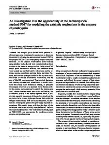
Figure 1: "One Way" displacements for strong motion and response records. Figure 1 shows the scatter of the "one way" sliding block displacements for different values of kc/km ratios. The data includes the strong motion records and the average seismic acceleration records. For the strong motion records only and for the acceleration ratios from 0.1 to 0.8, the scatter of the displacements is of 3

orders of magnitudes. When the average seismic acceleration records are added to the same data, the scatter increases to 4 orders and that too with only 20 such records. For the acceleration ratio of 0.9, the scatter increases to several orders of magnitudes. Sarma and Cossenas (2001) show that the scatter is much more when many response records are included. Therefore, the prediction based only on the kc/km ratio becomes meaningless. Following Sarma (1975) and Sarma(1988), the sliding displacements were normalized to [4u/kmgT2] where u is the sliding displacements and T is the predominant period of the records or the fundamental period of the dam. The normalization reduces the scatter to about 2 orders of magnitudes as shown in figure 2 and the relationship becomes: log [4u/kmgT2]= 1.17-4.07 kc/km

(1)

The standard error of this fit is σ= 0.51 with R2=0.81. This relationship compares reasonably well with that given by Sarma (1988). 1.00E+02 1.00E+01

u/(km.g.T^2)

1.00E+00 1.00E-01 0

0.2

0.4

0.6

0.8

1

1.00E-02 1.00E-03 1.00E-04 1.00E-05 1.00E-06 1.00E-07 kc/km

Figure 2: Normalised displacement as a function of the acceleration ratio A further attempt is then made to normalise the displacements by a factor dependent on the maximum velocity of the record, the average duration of the pulse (Tdn =dur/no) and the number of pulses n. The normalisation factor is given as: S= vmax(dur/no)m .n (2)

0.00E+00 0

0.2

0.4

0.6

0.8

1

log(u/S)

-1.00E+00 -2.00E+00 -3.00E+00 -4.00E+00 -5.00E+00 kc/km

Figure 3: Scaled displacement versus the acceleration ratios.

In this relationship vmax is the peak velocity of the record in cm/sec "dur", "no" and "n" are as defined before. The value of m is chosen to reduce the scatter. For a value of m=1, it was found that the scatter reduces to about an order of magnitude for smaller values of the acceleration ratios, as shown in figure 3. For the kc/km ratio of 0.9, even though the scatter reduces, it is still large. The examination of the data suggests that the value of m to reduce the scatter is different for different kc/km ratio. Instead of vmax, other parameters of the record such as amax , A95, Emax are also tried but the curve fitting is poor in terms of the standard error and the R2 value of the regression. Similarly, the use of the predominant period instead of the average pulse duration the curve fitting gives poorer results. The next stage of the analyses was performed for each kc/km ratios. The parameters chosen were the peak velocity, vmax, average duration of pulses, (t=dur/no), and the number of pulses, n, exceeding the critical. The number of pulses is important except for kc/km ratio of 0.9 and this is simply because, at this level, the no of pulse is 1 for almost all records. A regression analysis of the data in the following form is performed for each kc/km ratio. log (ucm)= C0 +C1 log vmax +C2 log Tdn + C3 log n

(3)

in which Tdn =average duration of pulses,= dur/no. vmax is in cm/sec. Figure 4 shows the very good fit of the data to the equation for kc/km=0.1. The fit is not as good for kc/km=0.8 but still acceptable. As can be seen from the standard error, the goodness of fit worsens as kc/km changes from 0.1 to 0.8. kc/km=0.1

Predicted log u

3 2 1 0 -1

0

1

2

3

-1 Computed log u

Figure 4: The computed and predicted log(u) for the acceleration ratio of 0.1 using peak velocity, average duration and the number of pulses. Table 3: Coefficients for the prediction of sliding displacements kc/km 0.1 0.2 0.3 0.4 0.5 0.6 0.7 0.8 0.9

C0 0.063 -0.090 -0.132 -0.182 -0.199 -0.237 -0.407 -0.556 0.633

C1 1.007 1.025 1.007 0.997 0.975 0.936 0.942 0.923 0.752

C2 1.061 0.998 1.016 1.032 1.077 1.146 1.221 1.327 2.347

C3 0.738 0.679 0.641 0.598 0.541 0.525 0.593 0.694 1.391

R2 0.988 0.984 0.979 0.977 0.976 0.948 0.936 0.906 0.805

σ 0.095 0.107 0.122 0.125 0.127 0.190 0.214 0.275 0.537

The results in table 3 show that the curve fitting for the acceleration ratio of 0.9 is again poor. Changing the vmax to amax for this particular set improves the standard error to 0.5. The relationship becomes: log (ucm)= -0.116 + 0.954 log amax + 2.751 log Tdn+ 1.945 log n (4) with R2=0.827 and Standard error σ=0.506. Since the number of pulses for kc/km ratio is mostly one, dropping the log(n) term from the regression, the equation becomes: log(ucm) = -0.019+ 0.875 log amax + 2.623 log Tdn (5) with R2= 0.778 and σ= 0.57 Closer examination of the data shows that at this level of acceleration ratio, even the shape of the pulse becomes important as can be seen from Sarma (1975, 1988) by comparing the triangular pulse with the half-sine pulse. The coefficients in table 3 for kc/km ratios of 0.1 to 0.8 are fitted to a relationship of the kind Ci = a0 +a1.(kc/km) +a2.(kc/km)2 ; 0.1 kc/km 0.8

(6)

The values of a0,1,2 are given in Table 4.

Co= C1 = C2 = C3 =

Table 4 a0 a1 0.033 -0.239 1.024 -0.031 1.097 -0.612 0.875 -1.264

a2 -0.561 -0.130 1.132 1.252

From the above study, it becomes apparent that over and above the knowledge of the peak acceleration and the peak velocity, some idea of the average duration and the number of pulses in acceleration records is necessary in order to predict the sliding displacements accurately enough. This therefore poses the problem associated with predicting sliding block displacements. For prediction purposes, in the absence of the record itself, the peak acceleration is known as the design parameter. Hazard analysis often provides the peak velocity of the expected record but not always. Sarma and Casey (1990) and Sarma and Srbulov (1997) showed that the "dur" and the "no" of strong motion records are related to A/A95 for each record. The present database shows a relationship between the peak acceleration and the peak velocity, which is given as: vmax = 0.07 kmg (7) with R2= 0.82 and standard deviation σ=0.019g. This relationship appears to be true for both the strong motion records as well as for the average seismic acceleration records obtained from the dam response analysis. A marginally better approximation is: vmax = 0.06 kmg + 0.028 gT (8) 2 with R = 0.85 and σ=0.017g. In the above two expressions, g is the acceleration due to gravity and it defines the dimension of vmax. Also T is the predominant period of the record or the fundamental period of the dam.

Peak Velocity (g.sec)

0.080000 0.070000 0.060000 0.050000 0.040000 0.030000 0.020000 0.010000 0.000000 0

0.2

0.4 0.6 0.8 Peak Acceleration (g)

1

Figure 5: Relationship between Peak velocity vmax and peak acceleration amax. The average duration, Tdn="dur/no" appears to be dependent on the predominant period T of the record and on the acceleration ratio kc/km, as shown in figure 6. kc/km=0.1

Average Duration of Pulses

0.2 0.15 0.1 0.05 0 0

0.5 1 Predom inant Period

1.5

Figure 6: Relationship between the average duration and the predominant period A linear regression gave the following results: Tdn= b0 + b1 T (9) Table 5: The coefficients for the relationship between average duration of pulse and the predominant period kc/km b0 b1 R2 σ 0.1 0.029 0.127 0.689 0.02 0.2 0.027 0.114 0.641 0.02 0.3 0.024 0.102 0.687 0.017 0.4 0.023 0.086 0.56 0.018 0.5 0.022 0.083 0.521 0.019 0.6 0.02 0.074 0.522 0.017 0.7 0.019 0.063 0.375 0.02 0.8 0.016 0.058 0.336 0.02 0.9 0.009 0.047 0.456 0.012 As before, the b0 and b1 values can be expressed as b0 = 0.0315 - 0.021 kc/km

(10)

b1 = 0.1319 - 0.0963 kc/km

(11)

and

The number of pulses, n, above a given acceleration ratio, kc/km, has no relationship to any of the strong motion parameters in the records. From the data base, the average number of pulses above an acceleration ratio is found and from this the relationship between the average number of pulses can be related to the acceleration ratio as: log (n) = 1.924 - 2.089 kc/km

(12)

The relationship of peak velocity with peak acceleration, the relationship of average duration of pulses with the predominant period and the acceleration ratio and the number of pulses with the acceleration ratio suggests a relationship of log u with the peak acceleration and the predominant period along with the acceleration ratio, as was suggested by Sarma (1975,1988). A further analysis is therefore performed to regress log u with the peak acceleration and the predominant period for each acceleration ratios. A linear regression equation of the following form is adopted. log ucm = S0 + S1log amax + S2 log T

(13)

Table 6 gives the values of the constants with the standard error and the R2 values. Table 6 kc/km s0 s1 s2 R2 σ 0.100 0.146 0.838 1.607 0.800 0.382 0.200 -0.214 0.828 1.615 0.822 0.353 0.300 -0.444 0.793 1.632 0.830 0.342 0.400 -0.691 0.768 1.629 0.832 0.336 0.500 -0.920 0.742 1.652 0.837 0.330 0.600 -1.102 0.692 1.715 0.820 0.352 0.700 -1.417 0.672 1.776 0.818 0.360 0.800 -1.886 0.669 1.846 0.767 0.432 0.900 -2.586 0.650 2.283 0.574 0.790 The goodness of fit of the data shown in figure 7 is obviously poor compared to that shown in figure 4. As before, for the acceleration ratio of 0.9, the fit is very poor. kc/km=0.1

Predicted log u

3 2 1 0 -1

0

1

2

3

-1

Computed log u

Figure 7: Computed and Predicted log u using peak acceleration and predominant period From the values in table 7, the following relationships can be derived which is valid for 0.1 S0 = 0.3862 - 2.6717 kc/km

kc/km (14)

0.8

S1 = 0.8728 - 0.2722 kc/km S2 = 1.6364 - 0.2703 kc/km + 0.6638 (kc/km)2

(15) (16)

The analysis performed above shows that the sliding block displacements can be predicted within about half an order of magnitude knowing the peak acceleration and the predominant period of the record or the fundamental period of the dam. If the duration and number of pulses can be predicted sufficiently accurately, the sliding block displacement prediction may be improved considerably. From the point of view of prediction, the acceleration ratio of 0.9 gives the poorest result but at this level of acceleration ratio, the actual displacements are very small and errors of one or even higher order of magnitudes is of no consequence. It is to be noted that replacing the predominant period by the fundamental period of the dam for the average seismic acceleration records may not be acceptable for periods greater than 1 second and further examination is therefore necessary. This will be dealt with in a future publication. THE VALIDITY OF THE SLIDING BLOCK MODEL IN EARTH DAM DESIGN The analyses incorporating the concept of the average seismic acceleration of sliding wedges and the sliding block model have been adopted worldwide in the seismic design of earth dams and embankments. This effect was based in the de-coupling approximation. The approximation assumes that the simplified procedure can be split into the following two tasks, Gazetas and Uddin, (1994): a. Perform an elastic dynamic analysis of the dam and obtain the spatial distribution of the response acceleration in the dam. This part assumes that no failure occurs. b. Use that distribution to assess the driving force on a possible sliding mass in a sliding block type of analysis. This part assumes that failure along a slip surface has no effect on the response accelerations of the dam. The concept of the model can be visualised as in figure 8. This is a simple model of a 3 degrees of freedom non-linear system.

up

u +ve M1 C1

M1 C1

K1

K1

M21 M22 C2

K2 x(t)

M21 M22 C2

K2 x(t)

Figure 8: A simple model to understand the sliding block model with the average seismic coefficient approach. Let us consider the model as displayed in figure 8. The model consists of three masses M1, M21 and M22. The masses M1 and M21 are connected by an elastic spring of stiffness K1 and by a damper of coefficient C1 as shown. The mass M22 is connected to the rigid base by a spring of stiffness K2 and a damper of coefficient C2. The masses M21 and M22 are in rigid plastic contact with limit strength F. The limit

strength for sliding in the left and right directions may be different thus causing the "one way" or the "two way" displacements. The motion of these masses can be described in two phases. In phase 1, when the two masses are in rigid contact, these form a single mass M2= M21 + M22 and the system behaves as a 20 of freedom system. When the net force above the contact exceeds the limit strength, the phase 2 of the 30 of freedom system begins when the mass M21 slides over the mass M22 causing relative displacement between the two. However, when the relative motion stops, the masses are stuck together again but leaving a yield displacement between the two sections of mass 2 and the motion reverts back to phase 1. Therefore the system shifts between a 20 and a 30 of freedom systems in time. We assume that the whole system is subjected to a ground shaking x(t). It is relatively easy to write the equations of motion for this two phase system and solve analytically. These equations and solutions are not shown here but some of the results are shown. We will call this solution the rigorous model representing the coupled solution. If on the other hand, we assume that there is no possible sliding between the masses and therefore responds in elastic mode only, then we can compute the average acceleration above the sliding surface. The limit strength provides the critical acceleration. The sliding block model is then applied to determine the permanent displacement, which represents the decoupled solution. Lin and Whitman (1983) have tested the validity of the de-coupling approximation, using a multi degrees of freedom lumped-mass model of a dam and solved the equations numerically. The permanent displacement calculated through this method is then compared to the de-coupled solution. They found that, in general, the decoupled approach provides conservative results for most practical cases. The largest overestimation occurs when the predominant period of the input is the same as that of the dam (i.e in resonance conditions). The error is higher for the case of deep wedges, and negligible for the case of shallow ones. They also found that for the kc/km ratio of nearly 0.5, and for a damping ratio of 0.15, the decoupled approximation overestimates the permanent displacement by about 20 %. Gazetas and Uddin (1994) have performed similar evaluation of the same issue, utilizing a finite element model to calculate the exact solution numerically, assuming a pre-existing potential sliding interface. The response acceleration records they produced for the case of the coupled analysis, exhibit some spikes at the end of each slipping phase. Those sharp spikes appear to be due to the additional dynamic excitation of the mass triggered by the reattachment of the sliding mass with the underlying body of the dam. The analysis has confirmed that the most severe overestimation of the permanent displacement by the decoupled method occurs when the dam is excited close to its resonant frequency. It is because, in the coupled method, build up of the response is drastically limited by the shearing strength of the interface, a constraint that is particularly effective at resonance. This is not the case for the de-coupled method where the driving acceleration is allowed to grow without limit, thus producing too high deformations, Gazetas and Uddin (1994). However their study again leads to the conclusion that the decoupled solution provides reasonable results for engineering purposes. Cascone and Rampello (2003), indicate that the de-coupled analysis has provided a very helpful tool for the design of an earth dam in Southern Italy. Wartman et al (2003) compared the coupled and decoupled displacements experimentally and found that the decoupled displacements may be non-conservative for some frequency ratios but this is because their reference ground motion is the base one. In the case of the soil column, the base motion is magnified near resonance. The simple system shown in figure 8 is used to determine the rigorous and the sliding block displacements for four strong motion records and the results are given in table 7. In this table, the values for the mass and stiffness were arbitrarily chosen to produce the first and second mode periods as shown. It can be seen that the method is more accurate for the higher values of the ratio kc/km. For low kc/km ratios, the sliding block displacements produce about 4 times higher displacements compared to the rigorous. This may be even higher for other records when the system may tend to resonate with the ground motion records. This accuracy is within the uncertainty associated with the prediction of sliding block displacements.

Table 7: Comparison of Rigorous and Sliding Block Displacements 1st Mode Period 2nd Mode Period Damping

0.64 sec 0.26 sec 10%

Average Original Seismic 0.1 Accn. Rigorous Sliding Record Amax Pred Period Amax Block g sec g cm cm Lp1 0.28 0.3 0.643 66.708 265.842 Lc1 0.16 0.16 0.062 3.924 8.195 Mv1 0.14 0.38 0.256 13.734 28.354 Iv1 0.16 0.3 2.807 570.942 2076.54

kc/km 0.4 0.7 Rigorous Sliding Rigorous Sliding Block Block cm cm cm cm 15.696 52.886 5.886 7.107 0.981 0.819 0 0.124 1.962 4.703 0.981 0.738 94.176 222 16.677 22.15

CONCLUSIONS Sliding block model provide an estimate of the displacements associated with slope failures within an accuracy of one order of magnitude even for very low acceleration ratios. The acceleration ratio as well as the number and the duration of pulses control the displacements. Comparison of rigorous and sliding block displacements shows good accuracy for engineering purposes. REFERENCES 1. 2. 3. 4. 5. 6. 7. 8. 9. 10. 11.

Ambraseys, N.N. and Menu, J.M. "Earthquake induced Ground Displacements." Earth. Eng. And Struct. Dynamics, 1988; 16, 6, 985-1006. Ambraseys,N. N. and Sarma, S.K. "The response of earth dams to strong earthquakes." Geotechnique, 1967; 25, 4, 743-761. Arias, A. "A measure of Earthquake intensity." Seismic Design for Nuclear Power plants, MIT Press, Cambridge, Massachusetts, 1970; 438-483. Cascone,E. and Rampello, S. "Decoupled seismic Analysis of an earth dam." Soil Dynamics and Earthq. Engrg.,Elsevier Science Direct, 2003; 23, 5, 349-365. Gazetas, G. and Uddin, N. "Permanent Deformation on Pre-existing sliding surfaces in Dams." J. Geotech. Engrg., 1994; 120, 11, 2041-2060. Lin J.S and Whitman, R.V. "De-coupling approximation to the evaluation of Earthquake-Induced plastic slip in Dams." Earthquake Engrg. And Struct. Dynamics, 1983; 11, 667-678. Makdisi, S.I. and Seed, H.B. "Simplified Procedure for estimating dam and Embankments earthquake-induced deformation." J. Geotch. Engrg. Div.,ASCE, 1978; 104, 7, 849-867 Newmark, N. M. "Effects of earthquakes on Dams and Embankments." Geotechnique, 1965; 15, 140-158. Sarma, S.K. "Seismic Stability of earth dams and Embankments." Geotechnique, 1975; 17, 181213. Sarma S.K. "Seismic response and stability of earth dams." Seismic risk assessment and design of building structures., Ed A. Koridze, Omega Scientific, 1988; 143-160. Sarma S.K. and Casey, B.J "Duration of strong motion in Earthquakes." Proc. 9th Euro. Conf. On Earthq. Eng., Moscow, 1990; 10-A, 174-183.

12.

13.

14. 15. 16. 17.

Sarma S.K. and Chlimintzas G. "Co-seismic and post seismic displacements of slopes." XV ICSMGE TC4 Satellite conf. "Lessons learned from recent strong earthquakes", Istanbul, Turkey, 2000; 183-188. Sarma S. and Cossenas G. "Dynamic response of dam layer systems to earthquake excitations." 4th International Conference on Recent Advances in Geotechnical Earthquake Engineering and Soil Dynamics, San Diego, California, 2001; Paper No. 5-19. Sarma, S.K. and Srbulov, M. "A uniform estimation of some basic ground motion parameters." J. Earthq. Eng., 1998; 2, 267-287. Sarma, S.K. and Yang, K.S. "An evaluation of Strong motion records and a new parameter A95." Earthq. Engng. And Struct. Dynamics, 1987; 15, 119-132. Seed, H.B. and Martin, G.R. "The seismic Coefficient in Earth dam Design." J.Geotech. Engrg.,ASCE, 1966; 92, 3, 25-28 Wartman, J., Bray, J.D. and Seed, R.B. "Inclined plane studies of the Newmark sliding block procedure." Journal of Geotechnical & Geoenvironmental Engineering, ASCE, 2003; 129, 8, 673684. Table 1: Data Base EARTHQUAKE

Code

Y

M D

Time

Station Name

Comp Amax (g)

vmax

Emax

a95

P. Per

(m/s)

(m^2/s)

(g)

(sec)

*

1 LYTLE CREEK

lc1

1970

9 12 14:30:53 DEVILS CANYON. CWR

180

0.164

0.071

0.695 0.133

0.16

2 LYTLE CREEK

lc2

1970

9 12 14:30:53 DEVILS CANYON. CWR

90

0.178

0.041

0.622 0.123

0.16

3 SAN FERNANDO

sf1

1971

2

9

6:01:00 SANTA FELICIA DAM

172

0.214

0.092

1.721 0.133

0.12

4 SAN FERNANDO

sf2

1971

2

9

6:01:00 SANTA FELICIA DAM

262

0.197

0.064

1.638 0.125

0.1

5 SAN FERNANDO

sf3

1971

2

9

6:01:00 FAIRMONT RESERVOIR

56

0.069

0.041

0.270 0.050

0.26

6 SAN FERNANDO

sf4

1971

2

9

6:01:00 FAIRMONT RESERVOIR

326

0.103

0.079

0.369 0.074

0.24

7 SAN FERNANDO

sf5

1971

2

9

6:01:00 GRIFFITH PARK OBS.

180

0.183

0.209

2.208 0.130

0.24

8 SAN FERNANDO

sf6

1971

2

9

6:01:00 GRIFFITH PARK OBS.

270

0.171

0.149

3.112 0.106

0.22

9 SAN FERNANDO

sf7

1971

2

9

6:01:00 LAKE HUGHES ARAY #4

111

0.196

0.057

1.322 0.114

0.12

10 SAN FERNANDO

sf8

1971

2

9

6:01:00 LAKE HUGHES ARAY #4

201

0.158

0.084

1.180 0.103

0.2

11 SAN FERNANDO

sf9

1971

2

9

6:01:00 LAKE HUGHES ARAY #9

21

0.125

0.048

0.750 0.074

0.14

12 SAN FERNANDO

sf10

1971

2

9

6:01:00 LAKE HUGHES ARAY #9

291

0.114

0.041

0.584 0.075

0.12

13 SAN FERNANDO

sf11

1971

2

9

6:01:00 LAKE HUGHES ARAY #12

21

0.357

0.164

5.502 0.263

0.18

14 SAN FERNANDO

sf12

1971

2

9

6:01:00 LAKE HUGHES ARAY #12

291

0.285

0.127

4.751 0.204

0.24

15 SAN FERNANDO

sf13

1971

2

9

6:01:00 CASTAIC OLD RIDGE

21

0.329

0.171

4.263 0.202

0.32

16 SAN FERNANDO

sf14

1971

2

9

6:01:00 CASTAIC OLD RIDGE

291

0.271

0.284

6.072 0.172

0.2

17 SAN FERNANDO

sf15

1971

2

9

6:01:00 CAL TECH SEISMO LAB

180

0.092

0.061

0.696 0.058

0.26

18 SAN FERNANDO

sf16

1971

2

9

6:01:00 CAL TECH SEISMO LAB

270

0.194

0.120

2.081 0.138

0.26

19 SAN FERNANDO

sf17

1971

2

9

6:01:00 SANTA ANITA RES. ARC

3

0.139

0.047

1.597 0.082

0.13

20 SAN FERNANDO

sf18

1971

2

9

6:01:00 SANTA ANITA RES. ARC

273

0.216

0.054

1.693 0.109

0.14

21 ALASKA

al1

1971

5

2

6:08:00 ADAK NAVAL BASE

NS

0.093

0.037

0.500 0.055

0.12

22 ALASKA

al2

1971

5

2

6:08:00 ADAK NAVAL BASE

EW

0.185

0.063

1.907 0.115

0.14

23 HOLLISTER

hol1

1974 11 28 23:01:00 GILROY ARRAY STN#1

247

0.144

0.051

0.304 0.104

0.1

24 HOLLISTER

hol2

1974 11 28 24:01:00 GILROY ARRAY STN#2

157

0.103

0.040

0.229 0.071

0.1

25 FRIULI

fri3_1

1976

5

6 20:00:13 TOLMEZZO-1

NS

0.366

0.229

4.835 0.243

0.26

26 FRIULI

fri3_2

1976

5

6 20:00:13 TOLMEZZO-1

WE

0.311

0.310

7.234 0.244

0.64

27 FRIULI

fri3_3

1976

5

6 20:00:13 TOLMEZZO-2

NS

0.100

0.040

0.208 0.082

0.24

28 FRIULI

fri3_4

1976

5

6 20:00:13 TOLMEZZO-2

WE

0.159

0.080

0.460 0.145

0.3

29 FRIULI

fri4_1

1976

5

7 23:49:00 TOLMEZZO-1

NS

0.128

0.038

0.193 0.101

0.1

30 FRIULI

fri4_2

1976

5

7 23:49:00 TOLMEZZO-1

WE

0.079

0.017

0.080 0.055

0.1

31 GAZLI

gaz1

1976

5 17

2:58:42 GAZLI

EW

0.730

0.700

29.751 0.454

0.15

32 FRIULI

fri1

1976

9 15

9:21:18 S ROCCO

NS

0.146

0.124

0.765 0.096

0.14

33 FRIULI

fri2

1976

9 15

9:21:18 S ROCCO

WE

0.238

0.188

1.413 0.173

0.2

34 FRIULI

fri3

1976

9 15

9:21:18 TARCENTO

NS

0.138

0.096

1.278 0.102

0.12

35 FRIULI

fri4

1976

9 15

9:21:18 TARCENTO

EW

0.110

0.040

0.762 0.080

0.12

36 FRIULI

fri5

1976

9 15

3:15:20 ROBIC.

NS

0.106

0.053

0.357 0.059

0.16

37 FRIULI

fri6

1976

9 15

3:15:20 ROBIC.

EW

0.075

0.037

0.278 0.043

0.1

38 FRIULI

fri2_1

1977

9 16 23:48:06 SOMPLAGO (U.G.)

NS

0.194

0.102

0.532 0.178

0.12

39 FRIULI

fri2_2

1977

9 16 23:48:06 SOMPLAGO (U.G.)

EW

0.100

0.030

0.180 0.070

0.12

40 TABAS

tabl1

1978

9 16 15:35:57 TABAS

N74E

0.873

0.187

9.947 0.199

0.17

41 TABAS

tab1

1978

9 16 15:35:57 DAYHOOK (IR)

N80W

0.369

0.251

10.044 0.239

0.4

42 TABAS

tab2

1978

9 16 15:35:57 DAYHOOK (IR)

N10E

0.398

0.888

70.239 0.545

0.24

43 MONTENEGRO

mn1

1979

4 15 14:43:00 HERCEG NOVI,SKOLA

NS

0.094

0.043

0.303 0.068

0.28

44 MONTENEGRO

mn2

1979

4 15 14:43:00 HERCEG NOVI,SKOLA

EW

0.081

0.031

0.217 0.056

0.26

45 MONTENEGRO

mn3

1979

4 15 14:43:00 ULCINJ-2

NS

0.171

0.187

3.728 0.118

0.52

46 MONTENEGRO

mn4

1979

4 15 14:43:00 ULCINJ-2

WE

0.230

0.280

4.550 0.159

0.72

47 MONTENEGRO

mn5

1979

4 15 14:43:00 HERCEG NOVI

NS

0.219

0.152

4.463 0.155

0.26

48 MONTENEGRO

mn6

1979

4 15 14:43:00 HERCEG NOVI

WE

0.251

0.117

2.745 0.152

0.3

49 MONTENEGRO

mn2_1

1979

5 24 17:24:00 KOTOR NAS,RAKITE

NS

0.122

0.076

0.886 0.080

0.22

50 MONTENEGRO

mn2_2

1979

5 24 17:24:00 KOTOR NAS,RAKITE

EW

0.154

0.089

1.208 0.102

0.4

51 COYOTE LAKE

cl1

1979

8

6 17:05:00 SAN MARTIN

250

0.246

0.205

2.211 0.207

0.38

52 COYOTE LAKE

cl2

1979

8

6 17:05:00 SAN MARTIN

160

0.139

0.114

1.153 0.101

0.38

53 COYOTE LAKE

cl3

1979

8

6 17:05:00 GILROY ARRAY STN#1

320

0.117

0.102

0.447 0.081

0.18

8

6 17:05:00 GILROY ARRAY STN#1

0.1

54 COYOTE LAKE

cl4

1979

230

0.087

0.040

0.336 0.054

55 IMPERIAL VAL.

iv1

1979 10 15 23:16:00 CERRO PRIETO

237

0.157

0.189

7.984 0.094

0.3

56 IMPERIAL VAL.

iv2

1979 10 15 23:16:00 CERRO PRIETO

147

0.167

0.117

7.068 0.107

0.32

57 IMPERIAL VAL.

iv3

1979 10 15 23:16:00 SUPERSTITION MT.

135

0.190

0.090

1.213 0.127

0.16

58 IMPERIAL VAL.

iv4

1979 10 15 23:16:00 SUPERSTITION MT.

45

0.114

0.046

0.513 0.064

0.16

59 ANZA

a1

1980

2 25 10:47:00 PINYON FLAT

135

0.085

0.022

0.144 0.065

0.09

60 ANZA

a2

1980

2 25 10:47:00 PINYON FLAT

45

0.127

0.050

0.288 0.110

0.08

61 MEXICALI VAL.

mv1

1980

6

9 10:00:00 CERRO PRIETO

45

0.143

0.135

0.839 0.096

0.38

62 MEXICALI VAL.

mv2

1980

6

9 10:00:00 CERRO PRIETO

315

0.104

0.084

0.602 0.073

0.3

63 VICTORIA

vi1

1980

6

9

3:28:00 CERRO PRIETO

45

0.556

0.324

11.666 0.338

0.22

6

9

3:28:00 CERRO PRIETO

0.14

64 VICTORIA

vi2

1980

315

0.599

0.197

5.861 0.193

65 IRPINIA

ir1

1980 11 23 18:34:52 BAGNOLI IRPINO

NS

0.133

0.214

2.220 0.094

0.18

66 IRPINIA

ir2

1980 11 23 18:34:52 BAGNOLI IRPINO

EW

0.187

0.325

2.740 0.121

0.12

67 IRPINIA

ir3

1980 11 23 18:34:52 STURNO

NS

0.223

0.388

7.992 0.157

0.38

68 IRPINIA

ir4

1980 11 23 18:34:52 STURNO

EW

0.305

0.670

9.285 0.201

0.2

69 IRPINIA

ir5

1980 11 23 18:34:52 CALITRI (A)

NS

0.157

0.253

6.532 0.094

1.26

70 IRPINIA

ir6

1980 11 23 18:34:52 CALITRI (A)

EW

0.172

0.297

8.327 0.098

0.34

71 IRPINIA

ir7

1980 11 23 18:34:52 VULTURE

NS

0.099

0.144

3.860 0.059

0.32

72 IRPINIA

ir8

1980 11 23 18:34:52 VULTURE

EW

0.098

0.075

2.883 0.056

0.22

73 WESTMORELAND wm1

1981

4 26 12:09:00 SUPERSTITION MT.

135

0.104

0.077

0.481 0.066

0.22

74 WESTMORELAND wm2

1981

4 26 12:09:00 SUPERSTITION MT.

45

0.082

0.036

0.221 0.045

0.08

75 MIRAMICHI, CAN mir1

1982

3 31 21:02:20 HOLMES LAKE

18

0.148

0.013

0.159 0.099

0.06

76 MIRAMICHI, CAN mir2

1982

3 31 21:02:20 HOLMES LAKE

288

0.175

0.016

0.265 0.105

0.04

77 MIRAMICHI, CAN mir2_1

1982

3 31 21:02:20 MITCHELL LK. RD.

L

0.124

0.012

0.144 0.079

0.04 0.04

78 MIRAMICHI, CAN mir2_2

1982

3 31 21:02:20 MITCHELL LK. RD.

T

0.206

0.021

0.317 0.145

79 MIRAMICHI, CAN mir2_3

1982

3 31 21:02:20 LOGGIE LODGE

L

0.172

0.017

0.290 0.118

0.04

80 MIRAMICHI, CAN mir2_4

1982

3 31 21:02:20 LOGGIE LODGE

T

0.342

0.044

0.520 0.231

0.04

81 MIRAMICHI, CAN mir3_8

1982

5

6 16:28:05 LOGGIE LODGE

T

0.109

0.011

0.036 0.094

0.04

82 MIRAMICHI, CAN mir3_7

1982

5

6 16:28:05 LOGGIE LODGE

L

0.108

0.023

0.086 0.098

0.08

83 ANZA

a2_1

1982

6 15 23:49:00 TERWILLIGER VALLEY

135

0.112

0.025

0.115 0.098

0.1

84 ANZA

a2_2

1982

6 15 23:49:00 TERWILLIGER VALLEY

45

0.091

0.041

0.112 0.072

0.12

85 COALINGA

coa1

1983

5

2 23:42:00 PARKFIELD,GOLDHILL 3W

90

0.123

0.091

0.956 0.087

0.3

86 COALINGA

coa2

1983

5

2 23:42:00 PARKFIELD,GOLDHILL 3W

0

0.138

0.117

1.001 0.097

0.38

87 MORGAN HILL

mh1

1984

4 24 21:15:19 COYOTE LAKE DAM

285

1.292

0.801

23.384 0.920

0.3

88 MORGAN HILL

mh2

1984

4 24 21:15:19 COYOTE LAKE DAM

195

0.701

0.512

17.253 0.480

0.28

89 MORGAN HILL

mh3

1984

4 24 21:15:00 GILROY ARRAY STN#1

320

0.091

0.029

0.339 0.055

0.14

90 MORGAN HILL

mh4

1984

4 24 21:15:00 GILROY ARRAY STN#1

230

0.072

0.028

0.287 0.035

0.08

91 MORGAN HILL

mh2_1

1984

4 24 21:15:00 SAN MARTIN.

285

1.293

0.801

23.387 0.920

0.3

92 MORGAN HILL

mh2_2

1984

4 24 21:15:00 SAN MARTIN.

195

0.701

0.512

17.255 0.480

0.28

93 LAZIO ABRUZZO

lz1

1984

5 11 17:49:41 ST.ATINA

NS

0.103

0.037

0.373 0.058

0.12

94 LAZIO ABRUZZO

lz2

1984

5 11 17:49:41 ST.ATINA

EW

0.109

0.036

0.319 0.066

0.24

95 LAZIO ABRUZZO

lz2_1

1984

5 11 10:41:50 ST.VIETTA BARREA

NS

0.151

0.064

0.725 0.097

0.16

96 LAZIO ABRUZZO

lz2_2

1984

5 11 10:41:50 ST.VIETTA BARREA

EW

0.220

0.095

0.910 0.154

0.18

97 LAZIO ABRUZZO

lz2_3

1984

5 11 13:14:57 VILLETTA BARREA

NS

0.138

0.070

0.253 0.122

0.28

98 LAZIO ABRUZZO

lz2_4

1984

5 11 13:14:57 VILLETTA BARREA

EW

0.088

0.043

0.107 0.069

0.18 0.3

99 LOMA PRIETA

lp1

1989 10 18

0:04:15 STANFORD, SLAC LAB

360

0.284

0.316

5.828 0.196

100 LOMA PRIETA

lp2

1989 10 18

0:04:15 STANFORD, SLAC LAB

270

0.203

0.383

3.586 0.140

1

101 LOMA PRIETA

lp3

1989 10 18

0:04:15 DIAMOND HEIGHTS, S.F.

90

0.113

0.147

0.652 0.076

0.46

102 LOMA PRIETA

lp4

1989 10 18

0:04:15 DIAMOND HEIGHTS, S.F.

0

0.097

0.107

0.860 0.075

0.32

103 LOMA PRIETA

lp5

1989 10 18

0:04:15 PRESIDIO, SF'CO

90

0.200

0.337

1.641 0.180

0.48

104 LOMA PRIETA

lp6

1989 10 18

0:04:15 PRESIDIO, SF'CO

0

0.100

0.135

0.956 0.074

0.72

105 LOMA PRIETA

lp7

1989 10 18

0:04:15 GILROY NO.1, GAVIALN

90

0.449

0.344

10.105 0.410

0.38

106 LOMA PRIETA

lp8

1989 10 18

0:04:15 GILROY NO.1, GAVIALN

0

0.408

0.313

6.192 0.327

0.2

107 TELIRE, LIMON

tel1

1991

4 22 21:56:00 SIQUIRRES STATION

NS

0.776

0.421

40.740 0.436

0.48

108 TELIRE, LIMON

tel2

1991

4 22 21:56:00 SIQUIRRES STATION

EW

0.271

0.233

8.818 0.171

0.4

109 FRAILES

fra1

1991

9

8

9:33:00 LA LUCHA

L

0.210

0.063

1.282 0.162

0.22

110 FRAILES

fra2

1991

9

8

9:33:00 LA LUCHA

T

0.260

0.098

1.891 0.184

0.24

Dam Response Record

Code

111 Tabas-L

tabLd1

112 Tabas-L

1978

vmax

Emax

a95

F. Per*

(g)

(m/s)

(m^2/s)

(g)

(sec)

Dam1

3.127

1.149 767.619 1.962

0.2

TabLd2

Dam2

2.513

2.049 601.923 1.640

0.4

113 Tabas-L

TabLd3

Dam3

2.419

2.102 581.493 1.492

0.6

114 Tabas-L

TabLd4

Dam4

2.625

2.427 725.061 1.644

0.8

115 Tabas-L

TabLd5

Dam5

1.696

2.046 453.207 1.133

1

116 Gazli

Gazd1

Dam1

2.033

0.797 201.198 1.261

0.2

117 Gazli

Gazd2

Dam2

2.027

1.267 376.129 1.436

0.4

118 Gazli

Gazd3

Dam3

1.914

1.434 229.270 1.210

0.6

119 Gazli

Gazd4

Dam4

1.414

1.192 168.035 0.987

0.8

120 Gazli

Gazd5

Dam5

1.204

1.189 132.515 0.886

1

121 Tabas1

Tab1d1 1978

Dam1

1.570

0.493 107.456 0.950

0.2

122 Tabas1

tab1d2

Dam2

0.998

0.548

93.528 0.618

0.4

123 Tabas1

tab1d3

Dam3

0.860

0.543

85.761 0.543

0.6

124 Tabas1

tab1d4

Dam4

0.807

0.547

60.562 0.525

0.8

125 Tabas1

Tab1d5

Dam5

0.516

0.504

48.797 0.346

1

126 Tabas2

Tab2d1 1978

Dam1

0.869

0.299

71.374 0.466

0.2

127 Tabas2

Tab2d2

Dam2

1.594

0.772 112.784 1.056

0.4

128 Tabas2

tab2d3

Dam3

0.893

0.662

95.282 0.574

0.6

129 Tabas2

tab2d4

Dam4

0.942

0.775

79.983 0.607

0.8

130 Tabas2

tab2d5

Dam5

0.780

0.750

68.026 0.548

1

1976

9 16

Amax

5 17

9 16

9 16

* P.Per= Predominant Period of the record *F.Period= Fundamental Period of the dam

Table 2:Sliding block displacements and other parameters dependent on kc/km (Representative only for one record) Record

Level Gr. Sloping Gr.

Code kc/km lc1

2-way

1 way

accn

u(cm)

u(cm)

(g)

a/a95

E

E/Emax

m^2/sec

dur

no

sec

Tdn=dur/no

n

sec

0.1

0.5971

2.7347

0.0164

0.1239

6.10E-01

0.878

1.906

52

0.036654

26

0.2

0.3871

1.5496

0.0328

0.2477

4.98E-01

0.717

1.167

26

0.044885

13

0.3

0.3359

0.9051

0.0493

0.3716

3.75E-01

0.54

0.779

19

0.041

10

0.4

0.2924

0.5325

0.0657

0.4954

2.60E-01

0.375

0.483

17

0.028412

9

0.5

0.2091

0.3144

0.0821

0.6193

1.79E-01

0.257

0.267

10

0.0267

5

0.6

0.1243

0.179

0.0985

0.7432

1.19E-01

0.171

0.167

6

0.027833

3

0.7

0.0718

0.095

0.1149

0.867

7.26E-02

0.104

0.117

3

0.039

2

0.8

0.0356

0.0405

0.1314

0.9909

3.58E-02

0.051

0.075

2

0.0375

1

0.9

0.0119

0.012

0.1478

1.1147

9.56E-03

0.014

0.041

2

0.0205

1