The Pennsylvania State University, Graduate Program in Acoustics, ... However, its physical meaning is not ..... [9] Blackstock, D.T., Fundamentals of Physical.
Investigation of a Single-Point Nonlinearity Indicator in One-Dimensional Propagation
Lauren Falco, Kent Gee, Anthony Atchley, Victor Sparrow
The Pennsylvania State University, Graduate Program in Acoustics, University Park, PA, 16802, USA , { lfalco, kentgee, atchley, vws1}@psu.edu
The influence of nonlinear effects in the propagation of jet noise is typically characterized by examining changes in the power spectral density (PSD) of the noise as a function of propagation distance. The rate of change of the PSD is an indicator of the importance of nonlinearity. Morfey and Howell [AIAA J. 19, 986-992 (1981)] introduced an analysis technique that has the potential to extract this information from a measurement at a single location. They develop an ensemble-averaged Burgers equation that relates the rate of change of the PSD with distance to the quantity Qp2p, which is the imaginary part of the crossspectral density of the square of the pressure and the pressure. With the proper normalization, geometrical spreading and attenuation effects can be removed, and the normalized quantity represents only spectral changes due to nonlinearity. Despite its potential applicability to jet noise analysis, the physical significance and utility of Qp2p have not been thoroughly studied. This work examines a normalization of Qp2p and its dependence on distance for the propagation of plane waves in a shock tube. The use of a simple, controlled environment allows for a better understanding of the significance of Qp2p. [Work supported by the National Science Foundation, the Office of Naval Research, and the Strategic Environmental Research and Development Program.]
1
Introduction
Morfey and Howell [2] derive an expression containing a quantity that has the potential to serve as a singlepoint nonlinearity indicator. A normalization of this quantity, often referred to as “Q/S” or “the MorfeyHowell nonlinearity indicator”, has recently been used by several researchers [1, 3, 4] in the analysis of highamplitude nose. However, its physical meaning is not well understood and has not yet been thoroughly investigated.
In the study of the propagation of jet noise, the power spectral density (PSD) is typically the quantity used to assess impact on the surrounding community. A correct assessment requires knowledge of whether the propagation is linear or nonlinear. If the propagation is nonlinear, the nonlinearity must be accurately accounted for in any prediction model. It has been shown [1] that, under some conditions, a linear propagation model does not accurately predict the evolution of the power spectral density of jet noise, especially for higher frequencies. The importance of nonlinearity is usually determined by examining the evolution of the PSD with propagation distance, a process that requires multiple measurements. However, nonlinearity is not the only factor that must be considered in the measurement and analysis of fullscale jet noise. Many other effects, such as wind and temperature gradients, ground impedance, and the spatial extent and directivity of the source influence the propagation of the noise. The complex nature of such an environment necessitates measurements (acoustic and meteorological) at many locations so that these effects can be quantified and selectively removed during analysis. In light of this complexity, it would be beneficial to be able to determine the presence or importance of nonlinearity with a measurement at a single location.
2
Theory
The present analysis follows that of Morfey and Howell [2]. Its basis is the Burgers equation,
∂p β ∂p δ ∂ 2 p − 3 p = , ∂x ρco ∂τ 2 ∂τ 2
(1)
where p is acoustic pressure, x is distance from the source, is the coefficient of nonlinearity, is ambient density, co is equilibrium sound speed, is retarded time, and is the diffusivity of sound [5]. The Burgers equation is frequently used as a model equation for nonlinear propagation because it includes both absorptive and nonlinear effects and because it has an exact solution. The authors next use a Fourier transform to write the equation in the frequency domain and generalize it for spherical spreading to obtain
1385
Forum Acusticum 2005 Budapest
Atchley, Falco, Gee, Sparrow
1 β ∂ + α ' r~p = jω 3 rq~ , 2 ρco ∂r
A physical interpretation of this equation can be drawn from the normalized harmonic amplitudes of an initially sinusoidal wave undergoing nonlinear propagation [6]. Figure 1 shows the fundamental along with the second, third, and fourth harmonics as a function of normalized distance for such a case. These are theoretical curves derived by Blackstock to connect the Fubini and Fay solutions. They are for plane waves and do not include any explicit atmospheric or boundary layer loss mechanism. The independent variable is distance normalized by the shock formation distance (also a quantity derived using the lossless plane wave assumption). Because these curves are plotted as a function of distance, the slope of a curve at any given point is qualitatively represented by the spatial derivative on the left-hand side of Equation (4). Thus, it appears that the fundamental and second harmonic will be of most importance near the source, and the higher harmonics will gain importance as propagation distance increases.
(2)
where r is radial distance from the source, is a generalized absorption and dispersion coefficient, ~ p is the Fourier transform of the pressure, and q~ is the Fourier transform of the square of the pressure. Multiplying Eq. (2) by the factor r times the complex conjugate of the transformed pressure and taking the ensemble-average of the real part yields
d 2 2αr β r e S p = −ω 3 r 2e 2αr Q p2 p , dr ρco
(
)
(3)
where Sp is the power spectral density and Qp2p is the imaginary part of the cross spectral density (also known as the quadspectral density) of p2 and p. Equation (3) is generalized for spherical spreading; however, the present experiments involve only plane waves, so the following form of the equation will be used:
d 2αx β e S p = −ω 3 e 2αxQ p2 p . dx ρco
(
)
3
(4)
3.1 Description
The term in parentheses on the left-hand side of Equation (4) is the absorption-corrected PSD. According to linear theory, the spatial derivative of this quantity should be zero. Thus, the right-hand side should account for any changes in the PSD due to nonlinearity. As it is written, a positive value for the right-hand side of Equation (4) indicates a gain of energy at that frequency and propagation distance; a negative value indicates a loss of energy at that frequency and propagation distance.
Normalized Amplitude
0.8 0.6 0.4
The data presented in this paper were obtained in a plane wave tube constructed of PVC pipe with an inner diameter of 5.21 cm and a wall thickness of 4.1 mm. The total length of the tube is 12.2 m, with 9.68 m available for acoustic measurements. The last 2.52 m contains a fibreglass anechoic termination consisting of a 1 m linear taper and a 1.52 m section of constant 28 kg/m3 density which attenuates frequencies of interest ( 2.9 kHz) at 100 dB/m [7]. Two JBL 2402H drivers are affixed to the opposite end of the tube using a “Tee” joint. Four B&K 6.35 mm type 4938 microphones are placed at 0.10 m, 3.25 m, 6.40 m, and 9.55 m from this joint, respectively. The first cross mode of the tube occurs at approximately 3.8 kHz. All data shown in this paper have a source frequency of 2.9 kHz. A schematic of the tube is shown in Figure 2.
Harmonic Amplitude Bn vs. σ
1
Experimental Apparatus
B1 B2 B3 B4
0.2 0 0
1
σ = x/xbar
2
3
Figure 1: Normalized amplitudes as a function of propagation distance for the first four harmonics of an initially sinusoidal wave Figure 2: Schematic of plane wave tube
1386
Forum Acusticum 2005 Budapest
Atchley, Falco, Gee, Sparrow
3.2 Validation
the agreement is sufficiently good for the preliminary investigations reported here.
In order to verify that sound in the tube consists of only travelling plane waves, that reflections from the termination are negligible, and that absorptive and nonlinear effects are as would be expected, measured waveforms and spectra were compared with numerical predictions. The prediction method used was a version of a code written by Gee [8]. The code is a hybrid time-frequency domain numerical solution to the Burgers equation for spherical waves that includes atmospheric absorption and dispersion. The version used here was created by removing spherical spreading and adding the effects of boundary layer absorption and dispersion [9]. To generate the predictions, the measured waveform from the first microphone (0.10 m from the source) was used as the input to the algorithm and propagated numerically to the other microphone locations.
Waveforms for 6.4 m, 136.9 dB re 20 µPa
Pressure (Pa)
200
-100
4
0.5
Time (ms)
1
1.5
Results
4.1 Nonlinearity Indicator The dependence of Qp2p on source amplitude and propagation distance was investigated by plotting the right-hand side of Equation (4) for various experimental conditions. For Figures 5 and 6, measurements from the first microphone (0.10 m propagation distance) were used to calculate Qp2p for four different source amplitudes.
Measurement Gee Code Prediction
2αx
d(e 4
0
2
80
Sp)/dx
0.10 m, 105.9 dB, σ = 0.0003 0.10 m, 140.9 dB, σ = 0.014
2
100
(Pa /(Hz*m))
PSD (dB re 20 µPa/rtHz)
0
Figure 4: Comparison of measured and predicted waveforms
PSD at harmonics, 6.4 m, 136.9 dB re 20 µPa
120
60
100
-200 0
Figure 3 shows the PSD of a measurement at the third microphone along with a numerical prediction for the same propagation distance. The source is a sinusoid at 2.9 kHz; values of the PSD for this frequency and its harmonics are shown. There is generally good agreement between the measurement and prediction, although the measured spectrum is somewhat less smooth than the prediction. This is probably a result of high-frequency scattering associated with the microphone holders. This kind of spectral variability is evident above 14 kHz in many of the measurements from the plane wave tube. 140
Measurement Gee Code Prediction
-2 5
10
15 20 25 30 Frequency (kHz)
35
40 -4
Figure 3: Comparison of measured and predicted power spectral densities
5
10
15 20 25 30 Frequency (kHz)
35
40
Figure 5: Normalization of Qp2p given by right-hand side of Equation (4) for two different (moderate amplitude) source conditions
Figure 4 shows the measured and predicted waveforms for the same case. Agreement here is also generally good, although the algorithm does overpredict the amplitude somewhat. This indicates the presence of additional losses from the tube that are not accounted for in the algorithm, such as sound radiation from the microphone ports or reflections at the joints. However,
1387
Forum Acusticum 2005 Budapest
2αx
d(e 100
The nonlinear growth of the higher harmonics begins to dominate as the propagation distance increases, especially at 9.55 m, for which the steepened waveform is shown in Figure 9. The spectral variability in Figure 8 is likely due to scattering and other irregularities in the sound propagation in the tube, as mentioned above.
Sp)/dx
0.10 m, 145.8 dB, σ = 0.025 0.10 m, 147.6 dB, σ = 0.031
50 0
2αx
d(e
2
(Pa /(Hz*m))
Atchley, Falco, Gee, Sparrow
1500
-50
10
15 20 25 30 Frequency (kHz)
35
1000
40
Figure 6: Normalization of Qp2p given by right-hand side of Equation (4) for two different (high amplitude) source conditions
-500
15 20 25 30 Frequency (kHz)
5
10
Pressure (Pa)
Sp)/dx
15 20 25 30 Frequency (kHz)
40
20 0 -20 -40 0
0.2
0.4
0.6 0.8 Time (ms)
1
1.2
1.4
4.2 Predictions Equation (4) was cast into the forward-difference form
35
β Q ( x) ρco3 p p 2
(5)
and used to propagate the PSD. Sp and Qp2p were measured at a distance x, and Equation (5) was used to predict Sp at a distance (x + x). This predicted PSD was then compared with the measured PSD at (x + x). Figure 10 shows one such prediction and comparison. In order to make this comparison with a measurement point, x must be equal to the distance between microphones on the plane wave tube, which is currently 3.15 m. In Figure 10, x = 6.40 m and (x + x) = 9.55 m, and the local sound pressure level at 9.55 m is 137 dB. The measurement and the prediction agree well for the first four harmonics, and the overall sound pressure levels agree to within 0.3 dB. The fact that the measured levels are generally higher than the
0.10 m, 147.6 dB, σ = 0.031 3.25 m, 145.9 dB, σ = 0.999
-500
35
Figure 9: Measured waveform corresponding to 139.7 dB at 9.55 m condition in Figure 8
0
-1000
10
S p ( x + ∆x ) = e − 2α∆x S p ( x ) − ω∆x
2
(Pa /(Hz*m))
500
5
Figure 8: Normalization of Qp2p given by right-hand side of Equation (4) for same source condition at third ( ) and fourth ( ) microphones
Figures 7 and 8 show the same quantity plotted for all four microphone locations at the 147.6 dB source condition seen in Figure 6. The sound pressure levels given in the legends are local to each microphone. While the value for the fundamental frequency is always negative, the (nonzero) values for the remaining harmonics are always positive, indicating that they continue to gain energy nonlinearly at all points along the propagation path. 2αx
500 0
A similar trend is present in these four data sets. In all cases, energy is being lost at the fundamental frequency and gained at the second harmonic frequency. This is consistent with the observations from Figure 1. It should be noted that although the values for the lowest amplitude case (105.9 dB in Figure 5) appear to be zero, they actually exhibit the same trend seen in the other plots but at an amplitude approximately four orders of magnitude less.
d(e
6.40 m, 142.5 dB, σ = 1.97 9.55 m, 139.7 dB, σ = 2.94
2
5
(Pa /(Hz*m))
-100
Sp)/dx
40
Figure 7: Normalization of Qp2p given by right-hand side of Equation (4) for same source condition at first ( ) and second (+) microphones
1388
Forum Acusticum 2005 Budapest
Atchley, Falco, Gee, Sparrow
References
predicted levels for the higher harmonics can be attributed to the continued growth of Qp2p at these frequencies between 6.40 m and 9.55 m. Overall, the agreement is good for this preliminary result, especially in light of the relatively large value of x.
PSD (dB re 20 µPa/rtHz)
130
[1] Gee, K.L. et al., “Preliminary analysis of nonlinearity in military jet aircraft noise propagation,” AIAA J. 43(6), 1398-1401 (2005).
Power Spectral Density
[2] Morfey, C.L. and G.P. Howell, “Nonlinear propagation of aircraft noise in the atmosphere,” AIAA J. 19(8), 986-992 (1981).
Measurement, 9.55 m, σ = 1.73 Prediction from 6.40 m, σ = 1.16
120
[3] McInerny, S.A., and Ölçmen, S.M., “Highintensity rocket noise: nonlinear propagation, atmospheric absorption, and characterization,” J. Acoust. Soc. Am. 117, 578-591 (2005).
110 100
[4] Petitjean, B.P. et al., “Acoustic pressure waveforms measured in high speed jet noise experiencing nonlinear propagation,” 43rd AIAA Aerospace Sciences Meeting and Exhibit, 2005, AIAA 2005-209.
90 80 0
10
20 Frequency (kHz)
30
40
[5] Lighthill, M.J., “Viscosity effects in sound waves of finite amplitude,” from Surveys in Mechanics, G.K. Batchelor and R.M. Davies, eds., Cambridge University Press: Cambridge, 250-351 (1956).
Figure 10: Prediction (+) from 6.40 m to 9.55 m generated using Equation (5), compared with the measured spectrum ( ) at 9.55 m
5
[6] Blackstock, D.T., “Connection between the Fay and Fubini solutions for plane sound waves of finite amplitude”, J. Acoust. Soc. Am. 39, 10191026 (1966).
Conclusions
An experimental apparatus has been developed to investigate the physical meaning and potential applications of the quantity Qp2p. This quantity has been identified as being related to the nonlinear distortion rate of a propagating finite amplitude wave. The normalization of Qp2p given by the right-hand side of Equation (4) has been shown to behave qualitatively as would be expected given the evolution of the harmonic amplitudes of an initially sinusoidal wave. Its dependence on source amplitude and on propagation distance have been demonstrated. Preliminary predictions using a finite-difference form of Equation (4) have been presented and have shown good agreement with measurements.
6
[7] Tarnow, V., “Measured anisotropic air flow resistivity and sound attenuation of glass wool,” J. Acoust. Soc. Am. 111(6), 2735-2739 (2002). [8] Gee, K.L. et al., “Nonlinear modeling of F/A-18E noise propagation,” 11th AIAA/CEAS Aeroacoustics Conference, 2005, AIAA 20053089. [9] Blackstock, D.T., Fundamentals of Physical Acoustics, John Wiley & Sons, Inc.: New York, 322-325 (2000).
Future Work
Work on the plane wave tube will continue with two goals: identifying and reducing excess losses and abnormalities in propagation; and adding the ability to vary the spacing of the microphones to allow for better accuracy in the determination of Qp2p and in predictions. Experiments will be performed in the tube with bi-frequency and noise sources, and the behavior of Qp2p for these cases will be investigated. These investigations may help to determine what value of Qp2p indicates the threshold of importance for nonlinearity and the dependence of Qp2p on distance.
1389