Investigation of Cue-based Aggregation in Static and Dynamic Environments with a Mobile Robot Swarm Farshad Arvin1,2
Ali Emre Turgut3
1
2
Tom´aˇs Krajn´ık4
Shigang Yue2
School of Electrical and Electronic Engineering, The University of Manchester, M13 9PL, Manchester, United Kingdom
Computational Intelligence Laboratory (CIL), School of Computer Science, University of Lincoln, LN6 7TS, United Kingdom 3
Mechanical Engineering Department Middle East Technical University (METU) 06800 Ankara, Turkey 4
Lincoln Centre for Autonomous Systems (L-CAS), University of Lincoln, LN6 7TS, United Kingdom
Contact person: Shigang Yue School of Computer Science University of Lincoln, Brayford Pool, Lincoln, LN6 7TS, United Kingdom E-mail:
[email protected]
1
2
Abstract Aggregation is one of the most fundamental behaviors that has been studied in swarm robotic researches for more than two decades. The studies in biology revealed that environment is a preeminent factor in especially cue-based aggregation that can be defined as aggregation at a particular location which is a heat or a light source acting as a cue indicating an optimal zone. In swarm robotics, studies on cue-based aggregation mainly focused on different methods of aggregation and different parameters such as population size. Although of utmost importance, environmental effects on aggregation performance have not been studied systematically. In this paper, we study the effects of different environmental factors; size, texture and number of cues in a static setting and moving cues in a dynamic setting using real robots. We used aggregation time and size of the aggregate as the two metrics to measure aggregation performance. We performed real robot experiments with different population sizes and evaluated the performance of aggregation using the defined metrics. We also proposed a probabilistic aggregation model and predicted the aggregation performance accurately in most of the settings. The results of the experiments show that environmental conditions affect the aggregation performance considerably and have to be studied in depth.
Keywords: Swarm Robotics, Aggregation, Collective Behavior, Cue-based aggregation
2
3
1
Introduction
Environment plays a crucial role in the daily routine and life cycle of all animals. Animals, their nests, behaviors and nutrition habits cannot be thought independent of the environment they live in. When we consider social animals such as ants, bees and termites environment becomes even more important in their daily routine. All the decisions they make are based on social interactions with their nest-mates and the state of the environment (Am´e, Halloy, Rivault, Detrain, & Deneubourg, 2006). Environment also serves as a medium for intraspecific communication (stigmergy) that is known to be a very effective way of communication in unstructured and complex environments (Schmickl & Crailsheim, 2004). Aggregation is a widely observed phenomenon in social animals especially in social insects (Gr¨ unbaum & Okubo, 1994). It can be defined as gathering of individuals into a single aggregate at a particular location. Aggregation behavior can be observed from amoeba (Rappel, Nicol, Sarkissian, Levine, & Loomis, 1999) to insects and to other animals (Camazine et al., 2001). Animals in an aggregate gain additional capabilities such as forming a spore-bearing structure by slime mold (Bonner, 1944), building a nest by termites (Parrish & Edelstein-Keshet, 1999) or protection against predators (Johannesen, Dunn, & Morrell, 2014; Morrell & James, 2008). Two different types of aggregation mechanisms are observed in nature: cue-based and selforganized (Camazine et al., 2001). In cue-based aggregation, animals aggregate on an external cue that is known to be an optimal zone for their survival; such as high temperature or high humidity zone for flies (Frank, Jouandet, Kearney, Macpherson, & Gallio, 2015). Self-organized aggregation does not require any external cues. Animals aggregate on some locations without any particular preference to their environmental conditions (Garnier, Gautrais, Asadpour, Jost, & Theraulaz, 2009). Cue-based and self-organized aggregation have been studied in swarm robotics for more than two decades (S¸ahin, Girgin, Bayındır, & Turgut, 2008; Brambilla, Ferrante, Birattari, & Dorigo, 2013; Bayındır, 2016). In cue-based aggregation, which is the main topic of this paper, one of the seminal works is due to Schmickl et al. (Schmickl, Thenius, et al., 2009). Inspired by honeybee aggregation in which bees aggregate on optimal temperature zones (Heran, 1952), Kernbach et al. (Kernbach, Thenius, Kernbach, & Schmickl, 2009) proposed a method known as BEECLUST for robot swarms. In BEECLUST, robots perform a random walk, and after a collision with another robot, they wait for a particular amount of time directly proportional to the intensity of the light
3
4
in the environment and then they continue doing a random walk. Many robots encountering with many others cause the swarm to aggregate on the optimal zone defined by the intensity of the light. Follow up works on BEECLUST mainly focused on: (1) modifications of parameters of BEECLUST to improve its performance (Arvin, Samsudin, Ramli, & Bekravi, 2011; Arvin, Turgut, Bellotto, & Yue, 2014), (2) derivation of simpler aggregation models based on systematic honeybee experiments (Schmickl & Hamann, 2011), (3) fuzzy-based aggregation methods for better aggregation performance (Arvin, Turgut, Bazyari, et al., 2014; Arvin, Turgut, & Yue, 2012), and (4) heterogeneity in behaviors (Kengyel et al., 2015). Although of utmost importance, to the best of our knowledge little has been done to study the effects of environment on aggregation. In this paper, we present a detailed study on effects of environmental changes on performance of a swarm system. We investigate different types of environments – static and dynamic – to check the influence of the changes on the performance of the bio-inspired aggregation mechanism based on the state-of-the-art BEECLUST algorithm.
2
Related Work
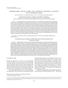
Study on honeybees’ thermotactic aggregation behavior is an early work on aggregation in biology (Heran, 1952) which showed that young honeybees tend to aggregate at an optimal zone with temperature between 34◦ and 38◦ C in a hive. The study revealed that bees follow a simple mechanism to form an aggregate based on two phases: performing a random walk until another bee is encountered and when encountered waiting for a certain amount of time based on the ambient temperature. Szopek et al. (Szopek, Schmickl, Thenius, Radspieler, & Crailsheim, 2013) studied the collective decision making of honeybees, which leads to thermotaxis-based aggregation at the optimal zone in a hive with a more systematic way. Their study revealed that a large group can find an optimal zone faster than the small size swarm. The results also showed that the group behavior is scalable and robust. In another study (Raveh, Vogt, Montavon, & K¨olliker, 2014), Raveh et al. showed that earwigs (Forficula auricularia) prefer to form aggregates with their relatives rather than other earwigs. This behavior helps to reduce the risk of competition between the individuals. In another interesting study (Broly, Devigne, Deneubourg, & Devigne, 2014), Broly et al. showed that aggregation helps woodlice colony (Isopoda: Oniscidea) to reduce water loss hence increase the survival rate of the colony. In case of mammals, a recent study on sea lions (Liwanag, Oraze1, Costa1, & Williams, 4
5
2014) revealed that sea lions tend to gather and form an aggregate when the ambient temperature reaches critical values. Aggregation helps them to decrease the heat transfer rate, hence keep their body temperature at the optimal level with lower energy loss. Therefore, during cold seasons, most of lions join the aggregate tightly instead of resting alone. Jeanson et al. studied cockroach (Blattella germanica) aggregation in a homogeneous environment (Jeanson et al., 2005). They showed that the probability of a cockroach to stop and wait in an aggregate depends on the size of aggregate. The bigger it is, the longer the waiting time is. On the contrary, Am´e et al. (Am´e et al., 2006) studied cockroach aggregation in a heterogeneous environment. Using two identical plastic shelters in an arena, they showed that cockroaches prefer to aggregate and rest under dark shelters. They figured out that the probabilities to join and to leave an aggregate are low when the population of the shelter is large. Although, this seems contrary to Jeanson et al. (Jeanson et al., 2005), it is not. In fact, larger aggregate reduces the probability of having access to the cue, hence this forms a negative feedback mechanism. In swarm robotics (Brambilla et al., 2013), self-organized aggregation has been performed in various studies. Trianni et al. (Trianni, Groß, Labella, S¸ahin, & Dorigo, 2003) presented an aggregation behavior using artificial evolution in two different settings: static and dynamic. In the static setting, when robots form an aggregate, they are not allowed to leave it, whereas in the dynamic setting, robots are allowed to leave the aggregate and join the other aggregates in the environment. In the static setting, it is observed that increasing the population size can result in formation of many separate aggregates. In the latter setting, robots in smaller aggregates have the chance to leave them and join the other ones, which finally results in formation of a single large aggregate. In another study, Soysal and S¸ahin (Soysal & S¸ahin, 2005) proposed a probabilistic aggregation mechanism based on simple behaviors as: obstacle avoidance, approach to an aggregate, repel from an aggregate, and wait. Performance of the system was investigated using various parameters including control strategies, time, and arena configuration. In a follow-up work (Soysal, Bah¸ceci, & S¸ahin, 2007), they also studied these parameters in aggregation using artificial evolution. In another study, Halloy et al. (Halloy et al., 2007) studied the aggregation behavior of a mixed group of robots and cockroaches in a two-shelter arena. The results revealed that the mixed group aggregated under the darkest shelter as expected. In a similar study, Garnier et al. (Garnier et al., 2008, 2009) used a miniature robot platform and implemented the behavioral model of cockroaches as proposed in (Jeanson et al., 2005). They were able to mimic the
5
6
aggregation behavior of cockroaches with robots in similar experimental settings as in (Jeanson et al., 2005). Campo et al. (Campo, Garnier, D´edriche, Zekkri, & Dorigo, 2011) proposed a collective decision making mechanism, which is based on the behavior of cockroaches, to discriminate between two different quality sources. The aim of the robots is to find the source that is the smallest, yet that can encapsulate the whole swarm. The experiments showed that the swarm was able to aggregate at the optimal source location and an increase in population size improved the performance of the swarm. In a recent study, Gauci et al. (Gauci, Chen, Li, Dodd, & Groß, 2014) proposed a self-organized aggregation mechanism with memory-less mobile robots with a binary sensor. The control mechanism includes: i) rotating on a spot when there is another robot and ii) circular backward movement when no other robot is detected. The results of simulated and real robot experiments showed that, robots tend to make a single aggregate using the proposed simple mechanism. However, to accomplish aggregation, the the binary sensor had to be able to detecto other robots at a long range. Kube and Zhang (Kube & Zhang, 1993) have performed one of the earliest studies in cue-based aggregation in swarm robotics. They proposed a collective transport scenario in which robots first aggregate around an object with a light source, and then push that object together. The aggregation method, which was used in that study is based on simple behaviors and does not rely on any explicit communication. To control the size of an aggregate in a cue-based aggregation scenario, Holland and Melhuish (Holland & Melhuish, 1997) proposed a mechanism, in which robots first aggregate around an infra-red transmitter, and then start to emit sound both synchronously and randomly. Therefore, each robot is able to estimate the aggregate size using the sound signal strength and decide to join and leave the aggregate accordingly. Mermoud et al. (Mermoud, Matthey, Evans, & Martinoli, 2010) used aggregation in a cue-based setting to enable a collective decision mechanism. Using a probabilistic aggregation method similar to the one in (Soysal & S¸ahin, 2005), robots first aggregate on a spot that could be either a bad spot (meaning that it should be destroyed) or a good spot (meaning that nothing should be done) and then they decide collectively whether to destroy or keep the spot intact. They showed that aggregation helps the robots to interact and communicate, which in turn helps them to make correct decisions under uncertainty due to noisy sensing. Francesca et al. (Francesca, Brambilla, Trianni, Dorigo, & Birattari, 2012) implemented the decision making strategy which cockroaches use in finding a resting shelter when there are more than one. They used a similar experimental setup which was
6
7
proposed in (Am´e et al., 2006). The results showed that, the probability of leaving an aggregate relies on the population and the capacity of the shelter. In a recent study (Schmickl & Hamann, 2011), Schmickl and Hamann worked on the aggregation of young bees as in (Heran, 1952) in a more systematic way. The results of real bee and robot experiments showed that bees follow a very simple set of behaviors for aggregation as: (i) A bee performs correlated a random walk. (ii) When a bee hits a wall, it avoids the wall and then continues to perform a random walk. (iii) When a bee encounters another bee, it stops and waits for a certain amount of time. Waiting time is directly proportional to the temperature of the spot. When the waiting time is over, the bee continues to perform a random walk. In another study (Kernbach et al., 2009), Kernbach et al. proposed an aggregation method called BEECLUST, which is based on honeybee aggregation as in (Schmickl & Hamann, 2011). The algorithm is based on robot-to-robot collisions as opposed to bee-to-bee encounters. In their setting, they assumed that there is a light source in the environment, which is used to crate a light gradient. Robots are required to aggregate on the zone where the intensity of the light is the highest. Each robot performs a random walk and stops when it encounters another robot. The waiting time of the robot depends on the intensity of the light where it stopped. The more the intensity, the longer it waits. After the waiting time is over, the robot turns to a random direction and restarts to perform a random walk. Through experiments they showed that robots are able to aggregate on the optimal zone. In a follow-up study (Schmickl, Thenius, et al., 2009), Schmickl et al. proposed two types of experiments. One is the static experiments in which there is a single light source as in (Kernbach et al., 2009) and the other is the dynamic experiments in which there are two light sources with different intensities and the intensities of the sources are changed during an experiment. Through systematic experiments, they showed that as in (Kernbach et al., 2009), robots were able to aggregate on the optimal zone in static experiments. Whereas, in dynamic experiments, robots are able to aggregate close to the highest intensity source and when the intensities of the two sources are switched during the experiment, robots are able to leave the previously formed aggregate and form a new aggregate under the recent optimal zone. Previously, we studied the effects of the different interactions among a group of robots and their decision making strategies. In (Arvin et al., 2011), we proposed two modifications on BEECLUST in order to increase its performance. One is the dynamic velocity in which robots are allowed to select three different speeds based on intensity of light; higher intensity results in slower speed
7
8
and vice versa. The other modification is the comparative waiting time. The waiting time of a robot increases in the presence of the other robots or aggregates. Both simulation-based and real robot experiments were conducted and results showed that both methods improve aggregation performance. In addition, we studied the effects of turning angle and its calculation methods on the performance of the swarm aggregation (Arvin, Turgut, Bellotto, & Yue, 2014). In that study, we compared the performance of two proposed aggregation algorithms – vector averaging and na¨ıve – with BEECLUST. The results showed that the proposed strategies outperform BEECLUST method due to additional environmental perception. In a recent study (Arvin, Turgut, Bazyari, et al., 2014), we introduced a fuzzy-based decision making mechanism in swarm aggregation and showed that the proposed method significantly improves the performance of aggregation using real-robot and computer-based simulations (Arvin et al., 2012). The rest of this paper is organized as follows. In Section 3, we introduce the aggregation method. Following that in Section 4, we introduce the proposed probabilistic model. In Section 5, we explain the realization of aggregation with real robots. In Section 6, we discuss the different experimental configurations and different experimental settings. In Section 7, we discuss results of the experiments in different settings. Finally, in Sections 8 and 9, we discuss the future research directions and make a conclusion of the study.
3
Aggregation Method
We use the state-of-the-art BEECLUST method (Schmickl, Thenius, et al., 2009). Fig. 1 shows the flowchart of the aggregation method. In this method, a robot moves forward continuously in the environment. When it encounters an object, it checks whether the object is an obstacle or another robot. If it is an obstacle, the robot avoids the obstacle and continues to move forward. If not, it stops and waits for a particular amount of time, the waiting time, w(t). The waiting time is a function of the ambient light intensity (Schmickl, Thenius, et al., 2009), which is estimated by the following formula:
w(t) =
60S(t)2 , S(t)2 + 5000
(1)
where S is the illuminance captured by the light sensor varying linearly from 0 and 255 corresponding to 0 lux and 600 lux. After the waiting time is over, the robot rotates ϕ degrees and continues
8
9
Figure 1: Finite state automaton that shows the robots’ behavior in BEECLUST.
to move forward. ϕ is a random variable drawn from a uniformly distributed set of angles in the range [−180◦ , 180◦ ].
4
Probabilistic Modeling of Aggregation
Stochastic characteristic of aggregation induce to use a probabilistic modeling scheme. To this end, several probabilistic models have been proposed in swarm robotics (Martinoli, Ijspeert, & Mondada, 1999; Lerman, Galstyan, Martinoli, & Ijspeert, 2001; Correll & Martinoli, 2007). Soysal and S¸ahin (Soysal & S¸ahin, 2007) proposed a macroscopic model of an aggregation behavior, which is able to predict the final distribution of the system. Bayındır and S¸ahin (Bayindir & S¸ahin, 2009) proposed a macroscopic model for a self-organized aggregation using probabilistic finite state automata, which could depict the behavior of swarm system appropriately. Hamann (Hamann, 2008) modeled the collective behavior of robots in a cue-based aggregation using a Langevin equation. Schmickl et al. (Schmickl, Hamann, Worn, & Crailsheim, 2009) proposed a macroscopic modeling of the cue-based aggregation using Stock & Flow model. In our previous work (Arvin, Attar, Turgut, & Yue, 2015), we proposed a mathematical model using a power-law equation to predict the aggregate size over time. In this work, to model the influence of the environmental parameters on the swarm behavior, we use a rate equation that represents the three processes that influence the size of an aggregate in single cue experiments. The equation is based on the probabilities of individual robots joining and leaving the aggregate during a given time interval. The rate of change of the number of aggregated
9
10
robots, na , can be expressed by means of these probabilities as:
n˙a =
dna = nf (2 pm + pj ) − na pl dt
,
(2)
where pj is the probability that a robot joins the aggregate, pm represents the probability that two non-aggregated robots meet on the cue, pl represents the chance that an aggregated robot leaves the aggregate and nf is the number of non-aggregated (free) robots. To calculate pj and pm , we have to find the chance that one robot detects another one during a given time interval. We based our approximation on an area that a single robot sweeps during a unit of time. Given that radius of the sensory system is rs and the robot radius is rr , two robots detect each other if their centers become closer than rs + rr . This means that during one second of movement with a speed of vr , a robot sweeps an area equal to as = (rs + rr ) vr . Given that the density of the non-aggregated robots excluding the subject robot is homogeneous and equal to (nf − 1)/aa , we can calculate the probability pm that two non-aggregated robots meet on the cue as:
pm = as
nf − 1 a c ac as = (nf − 1) 2 aa aa aa
,
(3)
where ac is the area of the cue and aa is the area of the arena. Similarly, we can calculate a probability pj that a non-aggregated robot meets an aggregated one as: pj = as
as na a c = na ac aa aa
,
(4)
where na is the number of aggregated robots, the na /ac is the density of the robots on the cue and ac /aa equals to the probability that the given robot is on the cue. To roughly estimate a probability that a robot leaves the aggregate, we take into account the waiting time w and the chance that it will not encounter another aggregated robot on the cue while leaving as: pl =
1 na as rc (1 − ), 2w ac 2vr
(5)
where rc /(2vr ) represents an average time it takes to leave the cue. A robot is also assumed to leave the aggregate when the dynamic cue on which the robots aggregated moves away. This means that the probability pl is increased by the chance that a robot has been in an area that the cue
10
11
left, leading to: pl =
1 na as rc vc (1 − )+ 2w ac 2vr π rc
(6)
where vc is the velocity of the dynamic/moving cue (see Section 6.2) and rc is its radius. Combining equations (3,4,6) allows us to express Eq.(2) as:
n˙a = nf
ac na na as rc na v c as (2 (nf − 1) + na ) − (1 − )− . aa aa 2w 2 a c vr π rc
(7)
Taking into account that nf +na = n, the rate of change n˙a can be fully expressed as a function of na , which allows us to calculate how the number of aggregated robots would change over time. Thus, it can be used to estimate the influence of certain parameters on the swarm behavior. Since a full analytic solution of this equation is beyond the scope of this paper, we created a Simulink model shown in Fig. 13 (see Appendix A) that allows us to change the model’s parameters and study their influence qualitatively. The proposed probabilistic model suggests that the rate at which the swarm aggregates increases quadratically with the population size: this means that a swarm with 3n robots would aggregate 9 times faster than a swarm with n robots. On the contrary, the area of the cue ac would have rather limited impact in the cue aggregation speed, because it mainly influences the aggregation speed in the initial phases, where pm ≫ pj . The model also suggests that increasing the sensor range rs and robot speed vr will both affect (through the as ) the aggregation speed in a (linearly) proportional way. In large populations, increasing or decreasing the waiting time should affect the steady number of the aggregated robots only marginally since the chance of a robot escaping the aggregate is low.
5 5.1
Implementation of Aggregation Robot Platform
We use Colias (Arvin, Murray, Zhang, & Yue, 2014) as our robotic platform in our experiments. It is specially designed for swarm applications. It is a small yet capable robot with a diameter of 4 cm. Colias is a compact version of AMiR (Autonomous Miniature Robot) (Arvin, Samsudin, & Ramli, 2009) with several additional functions enabling the implementation of wide range of swarm behaviors. Fig 2 shows a Colias robot and its modules. The robot has two boards – upper and
11
5.1 Robot Platform
12
lower – which have different functions. The upper board is for high-level tasks such as inter-robot communication and user programmed scenarios, however, the lower board is designed for low-level functions such as power management and motion control. Two micro DC gearhead motors and two wheels with diameter of 22 mm move Colias with a maximum speed of 35 cm/s. The rotational speed for each motor is controlled individually using pulse-width modulation (Arvin & Bekravi, 2013). Each motor is driven separately by a H-bridge DC motor driver, and consumes power between 120 mW and 550 mW depending on the load.
Figure 2: Colias micro mobile robot. The developed platform for swarm robotics research.
Colias uses IR proximity sensors to avoid collisions with obstacles and other robots and a light sensor to detect the intensity of the ambient light. The IR sensing system is composed of two different sub-units: The short-range sensing unit and the long range sensing unit. The short range sensing unit is composed of IR proximity sensors for immediate collision detection in a few centimeters. The long-range sensing unit is composed of six IR proximity sensors (each 60◦ on the robot’s upper board). It is used for obstacle and robot detection (Arvin, Samsudin, & Ramli, 2010). It is able to distinguish robots from obstacles within approximately 15±1 cm. Other than these sensors, Colias has a light (illuminance) sensor at the bottom facing down, which is used to detect illuminance on the ground (this will allow us to use a horizontally placed flat LCD screen as the ground on which robots move, explained in the following section). In Colias, the lower board is responsible for managing the power consumption as well as recharging process. Power consumption of the robot under normal conditions (in a basic arena with only walls) and short-range communication (low-power IR emitters) is about 2000 mW. However, it can be reduced to approximately 750 mW when IR emitters are turned on occasionally. A 3.7 V,
12
5.2 Arena Setup
13
Figure 3: Arena configuration including a 42” LCD screen as the ground and a mounted camera for recording/tracking the experiments.
600 mAh (extendable up to 1200 mAh) lithium-polymer battery is used as the main power source, which gives an autonomy of approximately 2 hours for the robot.
5.2
Arena Setup
To realize the aggregation experiments, we use rectangular arena with size of 90×57 cm2 . We employed a horizontally positioned 42” LCD screen as the ground on which the robots move. Fig. 3 shows the arena setup. In this way, we are able to create complex experiments with different settings with ease. All the aggregation cues, we implemented, are circular light spots with maximum illuminance of 420 lux, which are controlled by a PC. We use visual localization software developed in (Krajn´ık et al., 2014) to track the robots during experiments using an overhead camera. To reduce the amount of collected data from the localization system, we did not record all experiments in a video. Rather than that, a image of the arena was captured every 20 seconds.
5.3
Metrics and Statistical Analysis
We measure the performance of aggregation using the aggregation time, ta , and the size of the aggregate, na metrics. In order to define these two metrics, we need to first define the aggregation zone. The aggregation zone is defined as the area on the cue. A robot waiting on the aggregation zone is regarded an aggregated robot. The aggregation time is defined as the time that the aggregate size reaches at 70% of the total number of robots. The size of the aggregate is the total number of robots that are in the aggregate at a particular time of the experiment.
13
14
Table 1: Experimental values or range for variables and constants Values n na nf S w vr rs rr rc ar ag ac aa vc t ta t0 β
Description Population size Number of aggregated robots Number of free robots Sensor reading of illuminance Waiting time after collision Robot forward velocity Radius of robot IR sensory system Radius of robot Radius of cue Area covered by a robot Area covered by swarm Area of a cue Area of the entire arena Motion speed of cue Time Aggregate time when aggregation is accomplished Start of an aggregation scenario, t = 0 Ratio of the cue area to the area occupied by swarm
Range / Value(s) {9, 12, 15, 18} 0 to 18 robots 0 to 18 robots 0 to 255 0 to 65 sec 7 cm/s 3±0.3 cm 2 cm 12 to 22 cm 28 cm2 170 cm2 to 500 cm2 300 cm2 to 1500 cm2 0.51 m2 {1, 5, 10} mm/s 0 to 800 sec 0 to 750 sec 0 {2, 2.5, 3}
All results are statistically analyzed. We used analysis of variance (ANOVA) and the F-test method (Scheaffer, Mulekar, & McClave, 2010) in the analysis. F-test simply determines the degree of dependency between the selected parameters and results. A high F-value for a parameter means that it has more impact on the result. The standard values of the constants and variables, which are used in the experiments are listed in Table 1.
6 6.1
Experimental Setup Static Environment
In this set of experiments, we study the effects of several parameters; size, texture and number of the cue on aggregation performance in a static manner, i.e., we do not change the settings of an experiment once they are set. Each experiment is repeated with 9, 12, 15, 18 robots.
6.1.1
Size of Cue
In this setting, we study the effects of the different cue sizes on the performance of aggregation using a simulated gradient light, i.e. the brightness of the cue gradually decreases from its center. We assume that ar = πrs2 is the area that a robot has a sensing radius of rs during an instant of
14
6.1 Static Environment
15
Figure 4: (a) Area, ar , which a robot covers using its sensory system with radius of rs . (b) A cue implemented with gradient light with an area of ac relative to the number of robots, n, and β.
time (see Fig. 4a). Therefore, the total area which can be covered by radial arrangement of the robots is ag = nar , where n is the number of robots deployed in an experiment. In these experiments, we use three different sizes of cue for each population size, ac = β nar , β ∈ {2, 2.5, 3} (see Fig. 4b). We increase the size of the cue proportional to the population size. We set the cue sizes from a radius of 12 cm to 22 cm based on the population size and β. In robots, rs is defined to be 3 ±0.3 cm hence ar ≃ 28 cm2 . For example, in case of 9 robots, ag = 250 cm2 so with β = 2 the radius of the cue will be rc =12 cm, or in case of 18 robots and β = 3, ag = 540 cm2 hence the radius of cue will be about rc = 22 cm. 6.1.2
Texture of Cue
In these experiments, we study the effect of texture of the cue on aggregation performance. In particular, we formed two types of lighting conditions for the cue. One being the gradient type of lighting and the other being the non-gradient type of lighting. In the gradient cue, the luminance reduces gradually from the center to the edge of the cue, and in the non-gradient cue, the luminance is constant from the center to the perimeter.1 For each cue type, we used two different sizes. A small cue with a radius of rc = 16 cm (1.5 times larger than the area that can accommodate 18 robots) and a large cue with a radius of rc = 20 cm (2.5 times larger than the area that can accommodate 18 robots). 1 Heran et al. showed that honeybee aggregation is not only dependent on temperature itself, but also the temperature gradient around the optimal aggregation zone (Heran, 1952). In order to study this effect in our system, we change the texture, i.e., how light is distributed on the cue.
15
6.2 Dynamic Environment
6.1.3
16
Multiple Cues
In this setting, we study the effect of multiple cues with different sizes on the aggregation performance. In this regard, we used two gradient-type circular cues having different sizes. The main cue (Zone-1 with area of ac1 ) has a fixed radius of rc1 = 16 cm and the size of the second cue { } (Zone-2 with area of ac2 ) is set based on the size of the main cue as: ac2 = kac1 , k ∈ 13 , 15 . We track the size of the aggregate in both zones. Therefore, an experiment is terminated when the total number of robots (sum of all aggregate sizes) in both zones reaches 70% of the population size.
6.2
Dynamic Environment
In this setting, we change the position of the cue in different ways in order to create a dynamic environment. In particular, we study the adaptability of the swarm to dynamically changing environmental conditions. We created three different sets of experiments in order to test dynamic effects on aggregation performance effectively.
6.2.1
Switch Cue Location
In this experiment, a gradient-type cue with the radius of rc = 18 cm (which is 2 times bigger than the area that can accommodate 18 robots) is used as the aggregation zone. Each run takes 360 sec with three phases, each lasting 120 sec. This value was chosen based on the previous experiments (see Section 7.1) with similar population sizes, where the aggregation time never exceeded 120 s. In the first phase, the cue is placed on the left hand side of the arena. In the second phase of the experiment, the cue is moved instantly to the right hand side of the arena, and in the final phase the cue is moved back to the left hand side instantly. The experiment is performed with two different population sizes of 9 and 18 robots. We record the size of the aggregate during the experiments.
6.2.2
Delayed Motion
In this experiment, a single gradient-type circular cue with a radius of rc = 18 is used. The experiment includes two phases (stationary and moving) each lasting 120 s. In the first phase, the cue is placed on the left hand side of the arena and kept stationary and it starts to move with a
16
17
speed of vc = 3.5 mm/s continuously in the second phase.2 We repeat the experiment with 12 and 18 robots and we track the size of the aggregate with a period of 20 s.
6.2.3
Continuous Motion
In this setting, we use a single gradient-type circular cue with a radius of rc = 18 cm, which moves in a random direction continuously with a speed of vc mm/s, vc ∈ {1, 5, 10}. We repeat the experiment with 9 and 18 robots. During the experiments, we track the number of aggregated robots every 20 s.
7
Results
The results of the experiments are presented in this section. The results are depicted as box-plots. In the box-plots, boxes show the range of the first and the third quartiles of the data. Median of the data is shown with a horizontal line inside the boxes. The whiskers show the range between the minimum and maximum values of the data. A sample video of the swarm behavior and the experimental setup are provided online (Arvin, 2014).
7.1
Static Environment
Here, we depict the results of size of cue, texture of cue and multiple cues experiments.
7.1.1
Size of Cue
Aggregation time with respect to different cue sizes and number of robots is depicted in Fig. 5. We can see that for a fixed size cue an increase in the number of robots decreases the aggregation time. This effect is more preeminent when the number of robots is smaller. When we keep the number of robots the same, and change the size of the cue, we observe that larger cue size results in a shorter aggregation time. These observations are as expected. An increase in the number of robots increases the probability of collisions hence increases the probability to form an aggregate (provided that there is no 2 The
reason we chose the speed is that, if a robot encounters another one at a position where the light intensity is high, the robot is going to wait for 55 s. With rc = 18 cm, we guarantee that the waiting robot will not be on the cue after the waiting time is over, since the cue has already moved 19 cm during the waiting time.
17
7.1 Static Environment
18
overcrowding effect). On the other hand, an increase in the size of the cue increases the probability of successful collisions (meaning that the collision happened on the cue) hence increasing the probability to form an aggregate. Both resulting in a decrease in aggregation time.
Figure 5: Aggregation time in different population sizes at different cue sizes β ∈ {2, 2.5, 3}. The results of the proposed probabilistic model is depicted (shown in blue continuous line) together with size of cue results (here Fig 5 is redrawn for each β) as in Fig. 6. The model is able to predict aggregation time results both qualitatively and quantitatively.
Figure 6: Aggregation time in different β. Continues lines show the predicted aggregation size by the proposed model. We analyzed the results statistically. First, we used two-way ANOVA with factors of population and cue sizes to find the most effective factor on the aggregation time. We found that, the population size has more significant influence (P = 0.00, F = 81.73) than cue size (P = 0.07, F =
18
7.1 Static Environment
19
2.64) on the aggregation time. We then statistically analyzed the effects of cue size on each population, separately. The results showed that, the changes in cue size affect the aggregation time more in small population than the large population (F = {0.85, 0.72, 0.66, 0.51} for n = {9, 12, 15, 18}, respectively). Therefore, increase in population size compensates the fluctuations in the cue size.
7.1.2
Texture of Cue
The results of the experiments with a small cue (top) and a large cue (bottom) depicted in Fig 7. The predictions of the proposed model is also depicted on the same figure as a continuous blue line. In all the experiments, increase in the number of robots reduces the aggregation time. We can also observe that aggregation times with gradient-type cue is almost the same as the non-gradient-type cue. The only exception is the higher populations (with 15 and 18 robots) with non-gradient cue, which the swarm performance reduced in comparison to the same population size with gradient cue.
Figure 7: Aggregation time with gradient and non-gradient lights in different population sizes at (a) a small size cue (with radius of 16 cm) and (b) a big size cue (with radius of 20 cm). Continues lines indicate the predicted values from the probabilistic model.
19
7.1 Static Environment
20
Most of the results are in accordance with the expectations. An increase in the number of robots in any setting due to increase in the probability of collisions decreases the aggregation time. Here, we also see this effect. The type of lighting of the cue does not change the performance considerably. This was rather unexpected, but it could be due to geometrical constraints imposed by the size of robots and size of the cue. The proposed model is able to predict the results both qualitatively and quantitatively also in this case. We also analyzed the results statistically to see how aggregation time is dependent on the different factors. We checked the effects of population and texture of the cue as the factors and the aggregation time as the response (see Table 2). The results of the statistical analysis show that, in both cue sizes, the population size has significant impact on the aggregation time. However, the texture of the cue does not have a significant impact on the performance. We also analyzed the effects of cue size and population as two independent factors. The results of the statistical analysis revealed that, the population size is more effective (P