Dec 7, 2007 - Longmire & Marusic [6] where it was proposed that these hair- pin structures exist in packets and largely determine the prop- erties of turbulent ...
16th Australasian Fluid Mechanics Conference Crown Plaza, Gold Coast, Australia 2-7 December 2007
Investigation of velocity correlations in turbulent channel flow C. C. Chin1 , J. P. Monty1 , A. S. H. Ooi1 and I. Marusic1 1 Department of
Mechanical and Manufacturing Engineering University of Melbourne, Victoria, 3010 AUSTRALIA
Abstract
wall shear stress measurements are difficult to obtain.
Recently there has been an increase in studies pursuing a clearer understanding of the large-scale behaviour of wall-turbulence at high Reynolds numbers. These studies typically involve the analysis of a variety of statistics and correlations. In this paper, we investigate two-point cross-correlations of wall shear stress with various velocity components. These correlations have been calculated from two data sets: the Direct Numerical Simula´ tion (DNS) of a turbulent channel flow by Del Alamo, Jim´enez, Zandonade & Moser [2]; and experimental data from an extremely high Reynolds number atmospheric boundary layer, obtained from the SLTEST (Surface Layer Turbulence and Environmental Science Test) site at the great salt lakes, Utah. The experimental data were obtained by using sonic anemometers to measure all three components of velocity, and a novel wall shear stress sensor, developed by Heuer & Marusic [8]. The results provide further evidence of superstructures presented by Hutchins & Marusic [9] in the logarithmic region.
One important statistic that can be obtained from the correlation of U with τx is the inclination angle of the structures in the turbulent boundary layer. Investigations by Brown & Thomas [3] have shown that this inclination angle is approximately 18◦ . More recent studies carried out by Monty et al. [13] on the SLTEST data suggest a structure inclination angle of 15◦ . Measurements taken in that experiment will be used here. They include all velocity components, as well as the streamwise and spanwise fluctuating shear stresses, τx and τy . The velocity components were taken using 18 anemometers arranged in a 27m high array and a 100m wide horizontal array. The height of the sonic anemometers ranged from the lowest at z = 1.42m to the highest at z = 25.69m. The shear stresses were measured using a floating element shear stress sensor constructed by Heuer & Marusic [8]. The important parameters to note in the experiment were: Reθ = O(106 ), Uτ = 0.234m/s, where Uτ is the friction velocity in the streamwise direction, x. Other authors [9] have estimated boundary layer thickness, δ ≈ 60m, which is the boundary layer thickness used in this paper.
Introduction
Recently, there has been a concentrated effort by various research groups [5, 9, 13, 15], to calculate cross-correlations functions to gain a better insight into the fundamental mechanism of turbulent boundary layers. It is well known that vortical structures exist in turbulent boundary layers and they contribute to the transport of turbulent energy. Cross-correlation functions have proven to be an important tool as a methodology of identifying structures in the flow. This line of investigation was initiated by workers like Favre, Gaviglio & Dumas [4] and Grant [7] in the 1950s. The concept of hairpin-shaped structures in the turbulent boundary layer was first suggested by Theodorsen [14] and this idea has been extended recently by Adrian, Meinhart & Tomkins [1] and Ganapathisubramani, Longmire & Marusic [6] where it was proposed that these hairpin structures exist in packets and largely determine the properties of turbulent transport in the boundary layer. Later, the analysis of cross-correlation helped identify the existence of horseshoe or hairpin shaped structures, e.g. Willmarth & Tu [17], Moin & Kim [12]. More recently Ganapathisubramani et al. [5] have successfully used cross correlation functions to identify and study these hairpin vortex structures. Streamwise velocity correlations have been extensively studied by many investigators [5, 9, 12], using experimental measurements and numerical data. In this paper, we will define the three velocity components U,V and W (in the streamwise, x, spanwise, y, and wall normal, z, directions respectively), and the streamwise and spanwise fluctuating shear stress components, τx and τy . Analysis of streamwise velocity correlations involving U,V,W had been reported by Moin and Kim [12]. Spanwise velocity correlations of the U velocity component have been increasingly used to study and provide a better understanding between flow structures and eddying motions inside the turbulent boundary layer. Results from these studies have been presented in Moin & Kim [11], Tomkins & Adrian [15] and Hutchins & Marusic [9]. Studies of the streamwise cross-correlation with wall shear stress, τx are less common, mainly due to the fact that accurate
1436
The vast amount of information that can be obtained from DNS data has enabled scientists to gain a better understanding of the physics of the turbulent boundary layer. DNS data is especially useful to study the complicated motion and dynamics of the large-scale ‘superstructures’ (see Hutchins & Marusic [9]). The DNS data utilized in this paper is essentially the ´ same DNS data used in the study by Del Alamo et al. [2]. DNS were conducted at Reτ = Uτ δ/ν = 934, where δ is the half channel height. The size of the computation box is defined by Lx × Ly × Lz = 8πδ × 3πδ × 2δ. In this paper, we have computed cross-correlation coefficients between τx , τy and U,V and W from both the experimental measurements from the ASL (atmospheric surface layer) and DNS of a fully developed turbulent channel flow. The information will be used to expose the similarities and differences of the turbulent flow structures in these two data sets. To the authors knowledge, this is the first time that correlations between velocities and spanwise wall shear stress have been presented. Numerical Investigation Method
From the DNS data, cross correlation coefficients will be computed at z/δ values corresponding to the normalized heights of the sonic anemometers in the experiments conducted by Monty et al. [13]. The correlation analysis will be based on the fluctuating components which are denoted with lowercase letters, (ie. u, v and w). The cross-correlation between any two fluctuating components I and J is defined as, RIJ =
I(x, y)J(x + ∆x, y + ∆y) , σI σJ
(1)
where σ refers to the standard deviation and ∆x and ∆y are the spatial distances in the x and y directions. The overbar denotes the spatial average. From the correlations results, the structure
0.35
0.6
0.25 0.5
0.15 0.4 Rτ x u
0.05 −2
−1
0
1
0.3
0.2
0.1
0 −2
−1.5
−1
−0.5
0
0.5
1
∆x/δ Figure 1: Streamwise comparison of Rτx u showing z/δ ≈ 0.0237, 0.0357, 0.0500, 0.0710, 0.1023, 0.1452, 0.2087, 0.2990 & 0.4282 for both; DNS data, solid line (–); and ASL data, dashed line (−−). The inserted plot compares the Rτx u within the logarithmic region for DNS data of z/δ ≈ 0.1023 & 0.1452; and ASL data of z/δ ≈ 0.1023 & 0.1452.
inclination angle can determined by the following, θ = tan−1
z , ∆x peak
(2)
ing with the viscous length scale, ν/Uτ ). The peak correlations Rτx u for both DNS and ASL data are moving downstream of the measurement location with increasing z/δ. The DNS data of 25
where z refers to the wall normal height at which the correlation is calculated, and ∆x peak is the spatial distance difference where the maximum correlation occurs. For the experimental data, we have converted from time to space using Taylor’s hypothesis of frozen turbulence. That is ∆x peak = u∆t, where the convection velocity u is the mean velocity at the corresponding wall-normal position.
20 θ 15
Results and Discussion
For all the graphs presented, positive ∆x/δ corresponds to upstream of the measurement location and negative values correspond to downstream of measurement location. Figure 1 shows the correlations between τx and u for both DNS and ASL data with z/δ ≈ 0.0237, 0.0357, 0.0500, 0.0710, 0.1023, 0.1452, 0.2087, 0.2990 & 0.4282. Note that all following figures are plotted with the same z/δ values unless otherwise stated. Figure 1 shows an enlarged view of the ASL correlations (z/δ ≈ 0.1023 & 0.1452) comparing with the DNS correlations (z/δ ≈ 0.1023 & 0.1452), which correspond to the logarithmic region (100 . z+ . 140, where superscript ’+’ denotes scal-
10
5 101
102
103 z+
104
105
106
Figure 2: Structure inclination angle showing z/δ ≈ 0.0237, 0.0357, 0.0500, 0.0710, 0.1023, 0.1452, 0.2087, 0.2990 & 0.4282 for both; DNS data (△ ) and ASL data (◦).
1437
Rτx u suggest that the structure grows larger downstream in the x direction as z/δ increases from z/δ ≈ 0.0237 (z+ ≈ 23, for DNS data) to z/δ ≈ 0.4282.
0.1
In figure 2, structure inclination angles are compared for similar z/δ values as in figure 1. The average structure inclination angle for the ASL data is found to be θ = 14.2◦ . One should note that the average structure inclination angle for DNS data within the logarithmic region is found to be approximately 14.7◦ . The agreement is remarkable over such a Re range. The results support the findings of Marusic & Heuer [10] showing that the inclination angle of the structures is indeed invariant over the large range of Reτ .
0
Figures 3 & 4 show the correlations involving τx and w for both DNS and ASL respectively. Note that the abscissa scaling is different between figures 3 & 4. The difference in scaling provides a clearer image of the secondary peak present in the ASL data. It is interesting to note that even though the magnitude of the Rτx w is less for the ASL data, the general trend of the correlations is similar. Also note if we chose a certain z/δ and ∆x/δ location, the magnitude of |R| will be greater for |Rτx u | than |Rτx w |, this simply shows that there is a better correlation of u with τx further downstream, than w.
−0.1 Rτ x w −0.2
−0.3 −1.5
−1
−0.5
0 0.5 ∆x/δ
1
1.5
Figure 5: Decomposition of streamwise Rτx w using DNS data at z+ ≈ 34, actual Rτx w , solid line (–); small scale contribution + (λ+ x < 1000), dashed line,(−−); large scale contribution (λx > 1000), dotted line ( ). 0.1
An interesting finding in figure 3 shows the emergence of a secondary peak, however this peak occurs upstream of the measurement location. The secondary peak is also seen in ASL data. It was suspected that this secondary peak is a small scale
0 −0.1 Rτ x w
0
−0.2 −0.1 −0.3 −0.2 Rτ x w
−1.5
increasing z/δ
−0.3 −0.4 −2
−1
∆x/δ
0
1
Figure 3: Streamwise comparison of Rτx w using DNS data. 0.02
0
increasing z/δ
Rτ x w −0.02
−0.04
−0.06 −0.4
−0.2
0 ∆x/δ
0.2
0.4
Figure 4: Streamwise comparison of Rτx w using ASL data.
−1
−0.5
0 0.5 ∆x/δ
1
1.5
Figure 6: Decomposition of streamwise Rτx w using DNS data at z+ ≈ 137, actual Rτx w , solid line (–); small scale contribution + (λ+ x < 1000), dashed line,(−−); large scale contribution (λx > ). 1000), dotted line ( phenomenon rather than large scale. Hence a further investigation was carried out on Rτx w to determine if the secondary peak is contributed predominantly by small scale structures. From spectra analysis, the premultiplied u spectra peaks at λ+ x ≈ 1000 in the near-wall region, where λx is the streamwise wavelength. Therefore the value of λ+ x ≈ 1000 is chosen as the cut-off wavelength which determines the small scale structures. Figure 5 shows the correlation contributions of both the small and large scale structures at z/δ ≈ 0.0357. The correlation (solid line) at a given wall normal distance, z+ , shown is made up of the summation of two individual correlations, the small scale (dashed line), and the large scale (dotted line). The small scale structures are clearly responsible for the secondary peak even at greater wall normal distance (z/δ ≈ 0.1452) as shown in figure 6. From the contribution of the small scale structures shown in figures 5 & 6, a distinctive secondary peak is present. This suggests that there are even finer small scale structures present, where λ+ x ≈ O(100), that resulted in the secondary peak as seen in the dashed lines. The least contribution to the secondary peak + from the small scale structures (λ+ x < 1000) occurs at z = 15. The results suggest that the secondary peaks are mainly con-
1438
0.20
increasing z/δ
0.15
0.10
Rτ y v
0.05
0
−1
−1.5
−0.5
0
0.5
1
1.5
∆x/δ Figure 7: Streamwise comparison of Rτy v using DNS data, solid line (–); and ASL data, dashed line,(−−).
tributed by the small scale structures and small scale vortical structures are located around the large scale structures, even in the logarithmic region.
Figure 7 shows the correlations between τy and v where a secondary peak is also observed upstream. An enlarged view of 0.12
0.12
0.08
0.08
0.04 Rτ x v
Rτ y v
0
0.04
−0.04
0 increasing z/δ
−0.08
−0.04 −1.5
−1
−0.5
0 ∆x/δ
0.5
1
1.5
Figure 8: Streamwise comparison of Rτy v using ASL and DNS data for z/δ ≈ 0.1023 & 0.1452.
−1
−0.5
0 ∆x/δ
0.5
1
Figure 9: Decomposition of streamwise Rτy v using DNS data at z+ ≈ 34, actual Rτx v , solid line (–); small scale contribution + (λ+ x < 1000), dashed line,(−−); large scale contribution (λx > ). 1000), dotted line (
1439
0.30
0.4
increasing z/δ increasing z/δ
0.3
0.15
Rτx u 0.2
Rτ y u 0
0.1
−0.15
0 −0.3 −0.2 −0.1
0 ∆y/δ
0.1
0.2
−0.30 −0.3 −0.2 −0.1
0.3
Figure 10: Spanwise comparison of Rτx u using DNS data.
0 0.1 ∆y/δ
0.2
0.3
Figure 12: Spanwise correlations showing Rτy u using DNS data.
0.1
0.30
0
0.15
increasing z/δ
Rτ y w 0
−0.1 Rτ x w
−0.15 −0.2
increasing z/δ −0.30
−0.3 −0.3 −0.2 −0.1
−0.3 −0.2 −0.1 0 ∆y/δ
0.1
0.2
0.3
Figure 11: Spanwise correlations showing Rτx w using DNS data.
0 ∆y/δ
0.1
0.2
0.3
Figure 13: Spanwise correlations showing Rτy w using DNS data. 0.15
the ASL and DNS correlations is shown in figure 8, the z/δ values for the ASL and DNS data are the same as used in the inset in figure 1. Again both DNS and ASL correlations indicate secondary peaks. These peaks are again due to the small scale structures (shown in figure 9) which was shown using the same analysis carried out for investigating Rτx w in the streamwise direction. The general trend of the correlations between ASL and DNS are again similar. No significant correlations were found between τx and v, as well as τy and u, w, hence the results are not presented in this paper. The correlations in the spanwise direction involving τx and u, w are shown in figures 10 & 11 respectively. Both figures 10 & 11 display a peak correlation |Rτx ,u,w | at ∆y/δ ≈ 0. This is somewhat expected as the structures are not inclined or have minimal inclination in the spanwise direction. The correlations have a limited extent in the spanwise direction as compared to the correlations in the streamwise direction (figures 1 & 3). Another point worth noting is the abscissa crossover of Rτx w in figure 11. This identifies a region of alternating high and low velocity flow. This is consistent with (in an average sense) counterrotating vortex pairs. The next three figures 12, 13 & 14 display velocity correlations with τy in the spanwise direction. There is a crossover of the correlations from positive R to negative R in figures 12 & 13, which is always at the location ∆y/δ ≈ 0. This crossover feature provides further evidence of the existence of a pair counter rotating vortices. Such structures could be interpreted as the
increasing z/δ 0.10 Rτ y v 0.05
0 −0.3 −0.2 −0.1
0 ∆y/δ
0.1
0.2
0.3
Figure 14: Spanwise correlations showing Rτy v using DNS data. legs of the hairpin structure. Figure 14 shows a sharp drop in Rτy v at ∆y/δ ≈ 0 as z/δ increases and the occurrence of two distinct peaks is observed. One should note that Rτy v is symmetric about ∆y/δ = 0. The peaks are shifting outward away from ∆y/δ = 0 as z/δ increases. Figure 15 shows an enlarged plot of Rτy v at z/δ ≈ 0.0500, 0.0710 & 0.1023, and since the correlations are symmetric about ∆y/δ = 0, only the positive ∆y/δ region is shown. The spanwise length scales denoted by lz47 and lz96 correspond to wall normal distances of z+ ≈ 47 and 96 respectively. These spanwise length scales are a measure of the
1440
organization in the outer region of the turbulent boundary layer, Journal of Fluid Mechanics., 422, 2000, 1–54.
increasing z/δ
0.06
´ [2] Alamo, J. C. D., Jim´enez, J., Zandonade, P. and Moser, R. D., Scaling of the energy spectra of turbulent channels, Journal of Fluid Mechanics., 500, 2004, 135–144.
0.04 lz96
Rτ y v
[3] Brown, G. L. and Thomas, A. S. W., Large structure in a turbulent boundary layer, The Physics of Fluids, 20, 1977, S243–252.
0.02
[4] Favre, A. J., Gaviglio, J. J. and Dumas, R. J., Space-time double correlations and spectra in a turbulent boundary layer, Journal of Fluid Mechanics., 2, 1957, 313–342.
0 lz47 −0.02 0
0.1
0.2
0.3 ∆y/δ
0.4
[5] Ganapathisubramani, B., Hutchins, N., Hambleton, W. T., Longmire, E. K. and Marusic, I., Investigation of largescale coherence in a turbulent boundary layer using twopoint correlations, Journal of Fluid Mechanics., 524, 2005, 57–80.
0.5
Figure 15: Spanwise correlations showing Rτy v using DNS data for z/δ ≈ 0.0500 (z+ ≈ 47), 0.0710 & 0.1023. lz47 denotes spanwise length scale at z+ ≈ 47; lz96 denotes spanwise length scale at z+ ≈ 96.
[6] Ganapathisubramani, B., Longmire, E. K. and Marusic, I., Characteristics of vortex packets in turbulent boundary layer, Journal of Fluid Mechanics., 478, 2003, 35–46.
diameters of the vortical structures. Figure 15 clearly indicates that the spanwise length scales are shorter at near-wall region (lz47 < lz96 ) and the spanwise length scales of the vortical structures increase with the wall normal distance. The results suggest that the diameters of the vortical structures increase along the wall normal direction which agrees with the findings of Moin & Kim [12] and attached eddy hypothesis of Townsend [16].
[7] Grant, H. L., The large eddies of turbulent motion, Journal of Fluid Mechanics., 4(2), 1958, 149–190. [8] Heuer, W. D. C. and Marusic, I., Turbulence wall-shear stress sensor for the atmospheric surface layer, Measurement Science and Technology, 16, 2005, 1644–1649. [9] Hutchins, N. and Marusic, I., Evidence of very long meandering features in the logarithmic region of turbulent boundary layers, Journal of Fluid Mechanics., 579, 2007, 1–28.
Conclusions
An investigation of cross-correlations for DNS channel flow data and ASL data are presented. The structure inclination angle determined from the correlations using DNS data is very similar to that of the ASL data. The results suggest that in the streamwise direction of the flow, τx and τy are independent of each other, meaning that the velocity components u, v, and w will only exhibit a correlation between either τx or τy , the same comment cannot be made about correlations in the spanwise direction. The τy displayed correlations with all u, v and w in the spanwise direction. The only cross-correlation that did not show any significant result is between τx and v. The correlation plots have revealed more information about the behaviour of the structures in the spanwise direction. Information presented here clearly illustrates the existence of counter rotating pairs of vortical structures in the flow, even in the near wall region. Small scale structures are always present throughout the flow and contribute to the secondary peaks observed in the streamwise correlation results. Both DNS and ASL correlations provided evidence that the streamwise length scale is one order of magnitude greater than the spanwise length scale. The results and general trends of the correlations suggest that DNS is a suitable numerical method that can be utilized to provide good approximation of actual experiments over a large range of Reτ . Acknowledgements
The authors wish to gratefully thank Prof. R. D. Moser for making the Reτ = 934, DNS data available, and the financial support of the David and Lucile Packard Foundation and the Australian Research Council. References
[10] Marusic, I. and Heuer, W. D. C., Reynolds number invariance of the structure inclination angle in wall turbulence, Physical Review Letters in Press. [11] Moin, P. and Kim, J., Numerical investigation of turbulent channel flow, Journal of Fluid Mechanics., 118, 1982, 341–377. [12] Moin, P. and Kim, J., The structure of the vorticity field in turbulent channel flow. part 1. analysis of instantaneous fields and statistical correlations, Journal of Fluid Mechanics., 155, 1985, 441–464. [13] Monty, J. P., Chong, M. S., Hutchins, N. and Marusic, I., Surface shear stress fluctuations in the atmosheric surface layer, in Proceedings of the 11th Asian Congress of Fluid Mechanics, 2006. [14] Theodorsen, T., Mechanism of turbulence, in Proceedings of the 2nd Midwestern Conference on Fluid Mechanics., 1952. [15] Tomkins, C. D. and Adrian, R., Spanwise structure and scale growth in turbulent boundary layers, Journal of Fluid Mechanics., 490, 2003, 37–74. [16] Townsend, A. A., The structure of turbulent shear flow, Cambridge University Press. [17] Willmarth, W. W. and Tu, B. J., Structure of turbulence in the boundary layer near the wall, The Physics of Fluids, 10, 1967, S134–S137.
[1] Adrian, R. J., Meinhart, C. D. and Tomkins, C. D., Vortex
1441