Mar 9, 2018 - ABSTRACT. This paper presents the first results of a German study. (ITMA) that attempts to validate the GBAS CAT I ionosphere threat space ...
Attachment to NSP March 09 WGW/IPxx
Ionospheric Threat Model Assessment Christoph Mayer, Boubeker Belabbas German Aerospace Center DLR Winfried Dunkel DFS Deutsche Flugsicherung GmbH proportional to f −2 TEC , phase measurements are affected with reversed sign. Since GBAS is a differential system, not the absolute level of ionization is important but ionospheric gradients. The errors induced in GBAS by ionospheric gradients are dealt with as follows: o Nominal vertical ionospheric gradients are described by the parameter σ vig which is a
ABSTRACT This paper presents the first results of a German study (ITMA) that attempts to validate the GBAS CAT I ionosphere threat space that was developed for US CONUS. In phase 1 of this study the German Aerospace Center DLR and the German Air Navigation Service Provider DFS tried to determine the normal residual ionospheric uncertainty (σvig) and to identify periods with severe ionospheric activities relevant for GBAS. Dualfrequency RINEX data of up to 80 geodetic stations in and around Germany over an 11 year solar cycle from 1998 (25 stations) to 2008 (80 stations) was processed. Based on this data evaluation the study determined 16 periods with disturbed ionosphere in the years 2000 to 2003 and one day in 2005. These periods will be analyzed in more detail in phase 2 of the study to populate the GBAS CAT I ionosphere threat space. To determine the necessary parameters slope, velocity and width of the identified ionospheric fronts it is necessary to use additional GNSS data from German geodetic networks. This additional data should improve the resolution in the areas where the ionospheric front was detected. Phase 2 of the study should be completed in autumn 2009. The database may then be used to validate the assumptions regarding ionospheric effects for GAST-D.
parameter transmitted in the type 2 message of a GBAS ground station [2][3] o Anomalous ionospheric gradients are described by a threat model and can be mitigated, e.g., by geometry-screening methods [4][5][6]. Within the ITMA project both types of gradient information are determined for the region 2°E – 18°E, 45°N – 58°N (see Fig. 2). The data from an entire solar cycle 1998-2008 was processed. In the following some of the results obtained in phase 1 of the project are described in more detail. METHODOLOGY From dual-frequency GPS data, relative ionospheric range errors can be obtained from different combinations of observables
I phase _ diff =
f 22 (L1 − L2 ) f12 − f 22
(2)
I code _ diff =
f 22 (P2 − P1 ) f12 − f 22
(3)
I code− phase =
1 (P2 − L1 ) 2
(4)
INTRODUCTION The ionosphere is one of the error sources in groundbased augmentation systems. Usually, the ionosphereinduced errors in GBAS are small. However, very strong variations in the ionosphere plasma have been found which can compromise the safety of GBAS [4]. The total electron content (TEC) is given as the integral of the electron density along the ray path [7]
TEC = ∫ neds .
Here, L1 , L2 and P1 , P2 are the phase and code measurements on the two GPS-frequencies f1 , f 2 . All three combinations, Icode_diff, Iphase_diff, and Icode-phase are relative estimates of the ionospheric range error on the first GPS frequency, since they contain instrumentation offsets (e.g. differential-code-biases) and phase ambiguities. The relationship between TEC and these combinations is given by
(1)
The unit for TEC is 1 TECU = 1016 e m 2 . Since the ionospheric plasma is a dispersive medium, signals with different frequencies propagate in a different way. The effect of the ionosphere on the range measurements is
1
Attachment to NSP March 09 WGW/IPxx
I phase _ diff = 0.1623 × TEC + b ,
(5)
and analogously for Icode_diff and Icode-phase. Following the MOPS [2][3], the ionosphere is approximated as an infinitesimally thin layer at a fixed height hiono = 350 km. Slant and vertical ionospheric range errors are related by the so-called obliquity function
⎛ ⎛ r cos(elev ) ⎞ 2 ⎞ ⎟ ⎟ M (elev) = ⎜1 − ⎜⎜ E ⎜ ⎝ rE + hiono ⎟⎠ ⎟ ⎝ ⎠
velocity v slope g
−1 2
width W
(6)
Figure 1: The GBAS CAT-I ionosphere threat model
where rE denotes the earth’s radius and elev the elevation of the satellite. The relation between slant and vertical ionospheric range errors Islant and Ivert is
I slant = M (elev) ⋅ I vert .
data screening: identification of those time periods in 1998-2008 when anomalous ionospheric gradients have occurred in the considered region 2. threat-space determination: the parameters of the threat model have to be determined for all ionospheric fronts (with anomalous ionospheric activity) during the identified periods. Here, we report on the first step, the data screening. In order to identify periods of anomalous ionospheric activity, we have used the following gradient observable
1.
(7)
Determination of an over-bound of σ vig In order to determine an over-bound for σvig, we compute calibrated vertical ionospheric range errors Ivert,i and their ionospheric pierce points IPPi at a single epoch from a number of ground stations [7]. Then vertical ionospheric gradients vigi,j between each pair of measurements i,j may be computed as
vigi, j =
I vert ,i − I vert , j
(
dist IPPi , IPPj
)
,
distance
grad ROT =
I slant (t ) − I slant (t + Δt ) dist (IPP (t ), IPP (t + Δt ))
(9)
It is based on the time-difference of slant ionospheric range errors (“rate-of- TEC ”, ROT) within each data arc i.e. continuous measurements of a single pair of a groundstation and a GPS satellite. We used publicly available GPS data with Δt = 30s. As an estimation of Islant we used Iphase_diff, since this combination of GPS observables has the lowest noise contribution. Note that the unknown offset b cancels in the time-difference. In order to remove fake large gradients caused by bad data, e.g. cycle-slips, we have developed a suitable filter which rejects bad data points [1].
(8)
where the distance dist(IPPi,IPPj) between the ionospheric pierce points is computed at the height hiono. Since even small calibration errors in Ivert can generate large gradients at small IPP-distances, only pairs of measurements within the range 250km < dist(IPPi,IPPj) < 500km are used. Determination of anomalous ionospheric gradients Anomalous ionospheric gradients are taken into account in the GBAS integrity analysis by a threat model [5][6]. The threat model describes the worst-case ionospheric threat which is caused by moving ionospheric fronts. The threat space is determined from historical measurements. The anomalous ionosphere threat model has three dimensions, i.e. an ionospheric front is characterized by (see Figure 1) o slope g (mm/km=ppm) o velocity v (m/s) o width W (km). Unlike σvig, which quantifies vertical ionospheric gradients, the anomalous ionosphere threat model describes slant ionospheric range errors. In order to establish the threat model for a certain region, a minimal domain in its three-dimensional parameter space has to be determined. Within the ITMA project the following two-step process is used
RESULTS
We used data downloaded from SOPAC (Scripps Orbit and Permanent Array Center) and from BKG (Bundesamt für Kartographie und Geodäsie). For the period of 19982008 we determined the availability of GPS data in the region of interest which is indicated by the blue square in Figure 2. While in 1998 data from about 25 stations is available, the number of available stations increases and reaches about 80 stations in the year 2008. In order to determine σvig, we used data from different seasons and from different levels of solar activity, as indicated in Table 1; the number of used data points for each period is displayed in Table 2. The resulting complementary cumulative distribution functions of vertical ionospheric gradients for each period and the Gaussian over-bound for σvig = 2.07 mm/km is shown in Figure 3.
2
Attachment to NSP March 09 WGW/IPxx
Figure 3: CCDF for vertical ionospheric gradients: blue = winter, green = summer, solid lines = high solar activity, dashed lines = low solar activity. The dotted lines show the CCDF of Gaussian distributions with σvig =4 mm/km (red dots) and the over-bound σvig =2.07 mm/km (orange dots).
Figure 2 Available GPS-Stations from SOPAC and BKG
High Solar Activity Low Solar Activity (HSA) (LSA) winter 2001-001–2001-010 2007-154–2007-159 summer 2001-149–2001-158 2007-356–2007-363 Table 1 Vertical ionospheric gradients have been computed from 30s RINEX Data both for summer and winter periods in high- and low-solar-activity periods. The date format is YYYY-DOY. Season
Period HSA winter HSA summer LSA winter LSA summer
Number of used data points 114903 91630 322675 241245
Σ = 810273
Figure 4: In the top plot the number of data points is shown in blue, N100 (number of data points with gradROT >100 mm/km) in red and the number of excluded data points is displayed in green. The bottom plot shows the geo-magnetic AP and DST indices for the same period of time. For the year 2001 the resulting N100-values are shown in Figure 4, along with geo-magnetic indices [9] for the same period of time. It can be seen that anomalous ionospheric activities occur when the indices indicate a geo-magnetic disturbance. The converse statement, however, is not true, which is the reason for performing the data-screening with RINEX data instead of solely relying on geo-magnetic indices. In Figure 5, we show relative slant ionospheric delays and the corresponding gradROT -values for July 15, 2000 for a number of ground stations and the same GPS satellite G09. Note gradROT -values as determined by equation (9) are not corrected for the movement of the iono front. The plots are used to crosscheck the results based on time
Table 2: Number of used data points for σ vig .
Periods with anomalous ionospheric activity have been determined by analyzing 30s RINEX data for each day in 1998-2008 in the following way: o
Computation of gradROT -values from 30s RINEX data
o
Applying the gradROT -filter to the data in order to remove bad data points.
o
Determination of N30, N50, N100, N150, N200: the number of data points with gradROT > 30, 50, 100, 150, and 200 mm/km
o
If N100 > 1 and N50 > N100+1 the day is marked as a day with anomalous ionospheric activity.
3
Attachment to NSP March 09 WGW/IPxx difference of slant ionospheric range errors with the other combinations of observables mentioned ealier. Dentergem, Belgium
ACKNOWLEDGMENTS
We thank the SOPAC and BKG for providing RINEX data and Norbert Jakowski for providing calibrated vertical TEC data.
Helgoland, Germany
REFERENCES
[1] C Mayer, N Jakowski, T Pannowitsch, T. Dautermann, B. Belabbas, W Dunkel, ITMA Technical Note 1: Data-Screening, Feb 2009
Kootwijk, Netherlands
[2] Minimum Aviation System Performance Standard for the Local Area Augmentation System (LAAS), RTCA-DO245A, 2004
Westerbork, Netherlands
[3] Minimum Operational Performance Specification For Global Navigation Satellite Ground Based Augmentation System Ground Equipment To Support Category I Operations, ED-114, Eurocae, Paris, September 2003
Onsala, Sweden
[4] Pullen, Sam, Park, Youngshin, and Enge, Per The Impact and Mitigation of Ionosphere Anomalies on Ground-Based Augmentation of GNSS, Presented May 2008 at the 12th International Ionospheric Effects Symposium, Alexandria, VA; http://waas.stanford.edu/~wwu/papers/gps/PDF/Pulle nIES08.pdf
Worclaw, Poland
[5] Ramakrishnan, Shankar, Lee, Jiyun, Pullen, Sam, and Enge, Per, Targeted Ephemeris Decorrelation Parameter Inflation for Improved LAAS Availability during Severe Ionosphere Anomalies Presented January 2008 at the ION Institute of Navigation National Technical Meeting, San Diego, CA; http://waas.stanford.edu/~wwu/papers/gps/PDF/Ram akrishnanIONNTM08.pdf
Figure 5: The upper plot of each location shows relative ionospheric range errors Iphase_diff (red line), Icode-phase (blue line) and Icode_diff (green dots). The lower plot of each location shows the corresponding gradROT-values computed from Iphase_diff.
[6] Lee, Jiyun, Luo, M. Pullen, S., Park, Y. S., Enge, P., and Brenner, M. Position-Domain Geometry Screening to Maximize LAAS Availability in the Presence of Ionosphere Anomalies Presented September 2006 at the ION Institute of Navigation Global Navigation Satellite Systems Conference, Fort Worth, TX; http://waas.stanford.edu/~wwu/ papers/gps/PDF/LeeIONGNSS06.pdf
CONCLUSIONS
In the first phase of the ITMA project we have o determined an Gaussian over-bound for vertical ionospheric gradients σ vig =2.07 mm/km using calibrated vertical ionospheric range errors from periods of high- and low-solar-activity and from different seasons. o identified 16 periods with anomalous ionospheric activity by screening 30s RINEX data from 1998-2008 using up to 80 stations. For the second phase, the periods with anomalous ionospheric activity have to be analyzed with respect to the parameters in the threat model.
[7] Jakowski, N., TEC Monitoring by Using Satellite Positioning Systems, in Modern Ionospheric Science, (Eds. H. Kohl, R. Rster, K. Schlegel), EGS, Katlenburg-Lindau, ProduServ GmbH Verlagsservice, Berlin, pp 371-390,1996 [8] Jiyun Lee, Sam Pullen, Seebany Datta-Barua, and Per Enge, Assessment of Ionosphere Spatial Decorrelation for Global Positioning System-Based Aircraft Landing Systems, JOURNAL OF AIRCRAFT Vol. 44, No. 5, September-October 2007. [9] http://swdcwww.kugi.kyoto-u.ac.jp/dstdir/ http://www.ngdc.noaa.gov/stp/GEOMAG/kp_ap.htm l 4