IOWA STATE UNIVERSITY High School Employment, School Performance, and College Entry Chanyoung Lee, Peter Orazem June 2008
Working Paper # 08023
Department of Economics Working Papers Series
Ames, Iowa 50011 Iowa State University does not discriminate on the basis of race, color, age, religion, national origin, sexual orientation, gender identity, sex, marital status, disability, or status as a U.S. veteran. Inquiries can be directed to the Director of Equal Opportunity and Diversity, 3680 Beardshear Hall, (515) 294-7612.
High School Employment, School Performance, and College Entry
Chanyoung Leea Peter F. Orazemb
June 2008
The proportion of U.S. high school students working during the school year ranges from 23% in the freshman year to 75% in the senior year. This study estimates how cumulative work histories during the high school years affect probability of dropout, high school academic performance, and the probability of attending college. Variation in individual date of birth and in state truancy laws along with the strength of local demand for low-skill labor are used as instruments for endogenous work hours during the high school career. Working more hours during the academic year does not affect high school academic performance. However, increased high school work intensity raises the likelihood of completing high school but lowers the probability of going to college. These results are similar for boys and girls, and so working during high school does not explain the widening gap in college entry between men and women.
________________________
a
Institute for Monetary and Economic Research, The Bank of Korea
[email protected] Department of Economics, Iowa State University, Ames IA 50014-1070
[email protected] We thank the U.S Department of Labor for access to the NLSY 97 panel with geocodes, Agreement # 04-48
b
I. Introduction It is common for high school students in the United States to work during the school year.1 Data from the National Longitudinal Survey for Youth indicate that over the 1997-2003 period, the percentage of students who worked at least one week during the school year was 23% for freshmen; 45% for sophomores; 66% for juniors and 75% for seniors. This study examines whether working while in high school has any adverse consequences for school outcomes. With such high percentages of working students, many must feel that combining school and work is innocuous or even beneficial to children, at least for older children. Nevertheless, governments appear to believe there are adverse consequences for working at younger ages. The federal government limits the number of hours that children under 16 can work, and state and local governments may place additional age and hours restrictions on working youth. However, other state governments have concluded that combining school and work enhances human capital development, and have implemented programs to encourage working while in school in the belief that such programs improve school-to-career transitions. Academic studies have yielded inconsistent evidence regarding the effect of high school work on academic performance. One reason is that time allocated to academic performance and to work during the school year are joint decisions, suggesting that estimates must correct for the endogeneity of working while in school. It is highly likely that if children are doing poorly in school, working hours will be cut or curtailed entirely. On the other hand, students performing poorly in school may be more apt to seek work experience or on-the-job training opportunities to make up for weak academic training. Studies that ignored the endogeneity problem have come to various conclusions about the effects of working while in school on measures of school performance such as high school GPA, 1
Youth labor force attachment has been declining recently. The October labor force participation rate for 16- to 19-yearolds dropped over the 1994-2003 period from 50.4% to 42.2%. (Current Population Survey, Bureau of Labor Statistics)
1
dropout, or continuing education after high school. Among the studies with more positive outcomes from combining school and work, Steinberg et al. (1982) found either no correlation or a positive correlation between working while in school and Grade Point Average. Lillydahl (1990) reported that working up to 13.5 hours per week has a positive effect on GPA. Mortimer et al. (1996) found that high school seniors who worked less than 20 hours per week have higher grades compared to nonworking students. D’Amico (1984) concluded that school-year employment didn’t affect high school rank. Warren et al. (2000) found that working during high school didn’t affect curriculum choices or grades. D’Amico (1984) and Tienda and Ahituv (1996) reported that school work lowered the probability of dropping out. Other studies found harmful effects of school-year work on high school academic performance, particularly with more intensive work schedules. Greenberg and Steinberg (1986) reported that working over 20 hours per week lowers high school GPA. Stern (1995) found that working more than 15 hours per week has a negative effect on grades, time spent on homework and the likelihood of completion high school. Eckstein and Wolpin (1998) found a small negative effect on academic performance of employment during high school. Oettinger (1999) reported that working more than 20 hours per week lowers high school GPA of black and Hispanic youth but not of whites. Studies that correct for endogeneity have more consistently found adverse effects from combining school and work.2 Tyler (2003) examined the effect of working while in the last year of high school on twelfth-grade school test scores. When work is instrumented by variation in state child labor laws, he found a larger and significant decline in high school test scores relative to least squares estimates. Stinebrickner and Stinebrickner (2003) found that first-year college students randomly 2
Warren et al (2000) and Oettinger (1999) tested for but failed to find a reverse causal relationship in which academic performance influences on the employment during school. However, their tests of reverse causality will be biased if school attainment and work are jointly determined.
2
assigned to more demanding jobs lost about one-half of a grade point in first semester grades from working three hours more per week. Most studies of high school work and academic performance used the number of hours worked per week over a short time period, typically in the week or month prior to the interview date. Noisy or unreliable measures of time spent working could also explain the inconsistent results across studies. Of the exceptions, D’Amico (1984) generally found working regularly did not affect school performance regardless of work intensity. Ruhm (1997) found that working more intensively during high school increased earnings later in life. Both of these studies treat increased work intensity as exogenous, making it impossible to tell if their results might be due to unmeasured differences among students that cause some students to work more than others and that are also correlated with school performance or later earnings. Correcting for endogeneity, Rothstein (2007) found a small negative impact of current and past work while in school on high school GPA. This study extends the previous work by focusing on cumulative time spent working during the high school career; by examining multiple educational outcomes including academic performance, attaining a degree, and continuing to college; and by using plausible instruments to correct for the endogeneity of the time spent working. Consistent with Rothstein’s findings, more intensive employment experiences while attending high school have a small, negative and statistically insignificant effect on high school GPA. However, more intensive work reduces slightly the probability of high school dropout but also lowers the probability of attending college. A 10% increase in cumulative hours of work in high school leads to a 1.4% decreased likelihood of entering college. Nevertheless, despite the fact that boys work more hours than girls in high school, girls’ college entry is more adversely affected by work, and so working while in high school does not explain boys’ lower likelihood of entering college.
3
In the next section, we provide a model relating school performance and employment experience and validate instrumental variables. In Section III, we describe the data and present descriptive statistics. In Section IV, we provide empirical results and sensitivity analysis. In Section V, we summarize the policy implications of our findings.
II. Model In this section, we present a model that lays out the household choices and highlights the source of identification which we will utilize in the empirical work that follows. A. Theoretical background A household is comprised of a parent and a teenage child. The parent is assumed to make decisions so as to maximize household utility from consumption (C ) , and from the students’ school
performance (S ) . School performance is related to the child’s capacity for future human capital investments and earnings, and so S could be viewed as an index of expected future child wealth. The parent selects child time allocation and current consumption so as to maximize utility U=U (S, C). The child’s time, normalized to unity, is divided between schooling (TS ) and child labor (TW ) .3 The child’s school performance depends on the number of hours spent studying during high school and a vector of students’ individual, household, and community characteristics ( X ) . Numerous studies have shown that children with wealthier parents perform better in school. Child learning also depends on unobserved child’s individual ability or motivation ( μ C ) which may affect child time in school and work.
3
We are implicitly assuming that other uses of child time such as leisure consumption, household chores, or time spent on personal care (hygiene, sleeping, eating) are exogenous. Adding these activities into the model will not affect the reduced form solution to the optimization problem provided the opportunity cost of leisure or personal care time is the same as for schooling, and so we exclude these activities from the model for simplicity.
4
A high school student who works outside the household is assumed to earn an exogenous local market wage (WC ) . The parent’s labor supply is inelastic and yields an exogenous income (W A ) . The earned household income (W A + WC TW ) is used to purchase consumption goods at price normalized to unity and to purchase schooling that is priced at PS . The price of schooling is assumed to be altered by government policy on truancy age and age of school entry. For example, if state compulsory school attendance laws mandate that students living in the state must stay in school at an older age, the opportunity cost of schooling is lower because the option of working during school hours is removed. State policies on the minimum age at which children can enter school alter the average age and opportunity costs of schooling as well. Parents may be induced to send their children to private school to avoid age restrictions. Incorporating these various elements, the parent’s problem is to maximize U = U (C , S )
(1)
subject to the household budget constraint W A + WC TW = C + PS TS
(2)
and the school performance production function S = S (TW ,WA , μC , X )
(3)
Assuming interior solutions and considering child’s time constraint, the tradeoff between household consumption and educational investments on child is described by4 WC
∂U ∂U ∂S ∂U = −( + PS ) ∂C ∂S ∂TW ∂C
(4)
The parent allocates child time to school so that the marginal utility from current consumption purchased by the last hour of child time spent working is equal to the marginal utility from the last 4
In addition, concavity of the parents’ utility function implies that the educational production function has the usual properties: s ' > 0 and s ' ' < 0 with respect to time spent on studying.
5
hour of child time spent in school net of the lost utility from consumption. The solution of this problem yields a reduced form equation for child time spent in work: TW = T (W A ,WC , PS , X , μ C ) .
(5)
B. Empirical strategy
Our empirical work focuses on the linear approximations to equations (3) and (5).
TW = α 0 + α AWA + α CWC + α P PS + X 'α X + ε T
(6)
S = β 0 + βW TW + β AWA + X ' β X + ε S
(7)
where the error terms will be of the form ε k = γ k μC + ξ k ; k = T , S . Errors will have a component related to unobserved abilities and a purely random component. Ordinary Least Squares (OLS) will only yield a consistent estimate of school-year work on school achievement, βW in (7), if X and TW and are uncorrelated with the error ε S . But this will only happen if γ T = 0 in (6), which is unlikely given that μ C alters the optimal allocation of TW in (5). For example, suppose that teens with better endowments of μ C earn higher grade point averages. Suppose also that parents allocate child time to work activities only if they are doing well in school and so μ C and TW are positively correlated. Then the OLS estimate of the effect of work on high school GPA will be upward-biased. This could explain why some studies using OLS found no effect or even positive effects of school-year work on measured school achievement. Of course, the bias could go in the other direction if less able teens are more likely to work. We use an instrumental variables strategy to address the estimation problem. The theory suggests that factors that shift the value of child time, WC , or the price of child time in school, PS , will be good candidates for factors that shift the likelihood a child works but that do not directly affect schooling performance.
6
C. Instrumental variables
The strength of the local market for low-skilled labor is measured by average county retail sector earnings, as reported by the Bureau of Economic Analysis, during the period when the student is in high school. Higher average retail earnings should induce more high school students to work part-time while in school. Cameron and Taber (2004), Black et al (2005) and Rothstein (2007) found that local low-skilled earnings can significantly affect years of schooling across areas and time periods. Compared to other industries, the retail industry has the advantage that earnings and employment are reported for almost every county and that it is a heavy user of youth employees.5 As an example, eating and drinking establishments are the most common employers of high school aged youth (Rothstein, 2001). We use variation in legal restrictions on child time across states to approximate variations in the cost of child time in school. Every state stipulates an age at which students can legally leave school. The longer a child is required to stay enrolled in school, the less time potentially available for work. Students in states with lower dropout ages might be expected to work more during high school, if only because a young truancy age makes it more difficult for authorities to assess whether a working child is legally out of school. Similarly, restrictions on the age at which children can work suggest that children who enter high school at a younger age are less likely to work while in school. The Fair Labor Standard Act (FLSA) restricts work opportunities for children under the age of 16.6 Students who enter high school at older ages are not subject to the FLSA work limitations, although stricter state rules might still apply.
5
A variety of industries were investigated for inclusion such as agriculture, wholesale trade, service and construction suggested by Cameron and Taber (2004). 6 The Fair Labor Standard Act (FLSA) limits the number of hours and the type of work for 14- and 15- year olds. They may work outside school hours in various non-manufacturing, non-mining, non-hazardous jobs under the following conditions: no more than 3 hours on a school day, 18 hours in a school week, 8 hours on a non-school day, or 40 hours during a non-school week. Since age 14 is a typical starting age for high school, we can interpret the FLSA as allowing high school students to work with modest restrictions in terms of time and type of work.
7
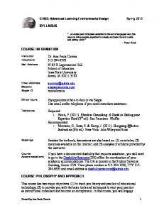
Similarly, the age at which a child enters high school may affect his decision to work. The expected age at grade 9 is computed based on the age entering 1st grade. In our sample, 68 % of students entered high school at age 14 and 25 % at age 15. All of these students can legally work while in high school and could drop out before completing high school, although when these laws take effect varied by age of the child and by the state in which the child resides. The legal drop out age by state is reported in Table 1 (National Center for School Engagement, 2003). Of the 43 states included in our sample, 26 states require students to remain in school until age 16; 5 states until age 17; and 12 states until age 18. Because school and work entry decisions are related to a child’s age, random variation in birth dates can affect the ages a child attends high school. If true, month of birth can affect the likelihood and intensity of working while in high school. Figure 1 shows the variation in the portion of students entering high school by ages 13 and 14, by birth month. Students born in the last quarter of the year are the most likely to enter high school by age 14 and many enter at age 13. Probability of early entry drops sharply for those born in the months before the start of the school-year. Those born in September are 25 percent more likely to enter school before age 15 than are those born in August.7 III. Data
The main data source for this study is the 1997 National Longitudinal Survey of Youth (NLSY97) consisting of 8,984 individuals born between 1980 and 1984. We make use of data up to the 2002 survey. To further concentrate on students who should have completed high school had they remained in school, we restrict the sample to students who enrolled in grade 9 by 1998 and who were born before 1984. Observations with missing values in key variables of this study are also excluded. Our working sample includes 3380 youths who obtained a high school diploma and 607 high school dropouts. 7
Angrist and Krueger (1991) and Tyler (2003) and Rothstein (2007) also used timing of birth to help identify years of schooling and child labor, respectively.
8
The NLSY97 collects retrospective employment data from the interview date back to the preceding interview date. This data include the beginning and ending dates of all jobs, all gaps in work within the same job and usual hours spent at work on each job. Based on this information, we generated weekly hours of work for each student both during the school year and in the summer. For some of our analysis, we also used aggregated work hours over time. The NLSY97 provides a wealth of useful information on household factors that may be correlated with labor market behavior and educational experiences. It includes gender, ethnicity, household income, family structure, parent’s highest education level, school performance and county of residence. Our analysis utilizes the restricted-use geocoded edition of the NLSY97 to identify each student’s county of residence. That allowed us to merge in indicators of local county labor market conditions and state compulsory schooling attendance laws. Table 2 reports weighted sample means of the variables used in the analysis, sorted by whether the individual is a high school dropouts; a terminating high school graduate; or a high school graduate who entered college. About 15% of the sample dropped out; 28% ended schooling with the high school degree; and 56% entered college after completing high school. As one would expect, the high school graduate subset performs better in school. High school graduates had average GPAs of around 3.0, whereas dropouts had average GPAs of 2.1.8 Employment intensity during the first two years of high school also differs between the two samples. On average, dropouts worked 180 hours more during the first two school years than did high school graduates who worked while in school. High school dropouts also worked around 75 hours more during the first summer of high school. Nevertheless, the summary data suggests other reasons why more intense work might be correlated with dropout. Dropouts come from poorer households than do high school graduates, and so the 8
The NLSY reports high school grades on a scale from 0 to 13. These scores correspond to approximate grades such as “mostly C” or “mixed A with B” and so on. These approximate grades were converted into a 4.0 scale. “Mostly C” is converted to 2.0 and “Mixed A with B” is converted to 3.5.
9
higher work hours of dropouts may reflect other observable or unobservable differences between the two samples. IV. Empirical Results A. Labor supply while in high school
We are relying on our labor supply equation (6) to identify school-year working hours in our human capital production equation (7). We first demonstrate that our child labor supply shifters can significantly influence hours of work while in high school. Research has demonstrated that instruments that are only weakly associated with the endogenous variables invalidate the estimation method (Bound et al. 1995). We regress cumulative hours of work during high school on the expected age at which students enter high school, the legal drop out age by compulsory schooling attendance laws in state, local average earnings per worker in retail industry during their high school year, month at which students were born, the square of the month, and a number of other control variables. For comparison purposes, the first column of Table 3 contains the regression incorporating only the vector of exogenous control variables. The first and second rows in column 2 of Table 3 show month of birth has a quadratic relationship with hours of work during high school. Cumulative hours are decreasing in month of birth until June, but then increase for students born in the second half of the year. The difference apparently reflects how birth month affects the probability of entering high school at a young age. As shown in Figure 1, the probability of entering high school before age 15 rises from September through April and then falls thereafter. Entering high school at an older age has a dramatic effect on child labor supply: delaying age of entry by one year raises cumulative hours worked in high school by 50.7%. Black and Hispanic children are less likely to work than white children with similar home situations. However, poverty does influence child labor. Probability of working decreases as
10
household income and parental education increase, while children from single-parent homes work more. In the third column, legal dropout age is included. Individuals in states with truancy ages one year older work 12% fewer hours during high school. The fourth column shows that adding local earnings to the third column specification increases the model’s explanatory power. Average county retail earnings of students’ school year have a positive and significant effect on hours worked in high school. A 10% increase in average retail earnings increases cumulative hours of work while in school by 8% on average. The null hypothesis that the coefficients on the set of instruments used are jointly zero can easily be rejected with an F- statistic of 9.9, providing evidence that local labor market conditions, birth month and compulsory schooling attendance laws can shift significantly the intensity of high school students’ work. It also appears that these instrumental variables are not directly correlated with school performance. Though it is not a definitive test, the fifth column of Table 3 provides the results when high school grade point average is regressed on individual characteristics and the instrumental variables used in this study. We failed to reject the null hypothesis that the instruments have no joint influence on grades at standard levels of significance. B. Impact of working while in school on school outcomes
Table 4 presents the OLS and IV estimates of β from equation (7). The estimated effect of employment on schooling outcomes is shown in the first row of each column. The OLS estimate of the direct academic performance effect of work during high school year is very small but statistically significant. It implies that a 10 % decrease in cumulative hours of work during high school would increase high school GPA by around 0.02.9
9
The calculation is based on ∆ HS GPA
≅ (
β 100
) (%∆ Work hours). 11
The IV estimates in the second column are obtained when labor supply during high school is instrumented by expected age entering high school, the month of birth, and the square of the month. It shows that the IV point estimate of having a part time job is nearly twice as large as the OLS estimates in absolute value but is not significant. The literal interpretation is that a 10% increase in hours worked during high school lowers high school GPA by 0.039 points. The same results are obtained when we use different sets of instruments.10 Both OLS and IV estimates indicate that cumulative hours of work during high school do not greatly hamper high school academic performance.11 The results also show that, holding family background fixed, girls outperform boys by 0.25 points in high school GPA. Gaps of comparable magnitude are found between Whites and Blacks or Hispanics. Living with richer and better educated parents raises GPA substantially with an average 0.8 points difference between students with college educated parents compared to students with high school educated parents. To put the child labor effect in perspective, two years of parental education more than compensates for the lost GPA from working 10% longer hours in high school. Since we have more instruments than endogenous variables, our model is over-identified. The test of over-identifying restrictions produces a χ2 statistic of at most 3.81. Thus, we fail to reject the null hypothesis that the instruments are uncorrelated with the error term. The same approach used above is applied to examine the effect of work during high school on the likelihood of attending college. Table 5 presents the probit estimates and two stage probit estimates. The marginal effects are reported as evaluated at the mean of each variable. The uncorrected estimate treating work hours as exogenous suggests that a ten percent increase in hours
10
Various definitions of birth month were tried. For example, instead of numbering months starting in January, an alternative specification numbered the months starting in September to reflect the school year. Another alternative replaced the numbered months by a series of 11 birth month dummy variables. Results are invariant to the definition used. 11 Similar effects of work on academic performance were found for male and female youth.
12
worked during high school decreases the probability of entering college by 0.2%, a statistically significant but numerically small effect.12 The IV estimates obtained using a two stage probit correcting for the endogeneity of labor supply finds a more substantial effect. A 10 % increase in employment intensity during high school lowers the probability of college entry by about 1.4%. Other things equal, women are 1.3 percent more likely to enter college than men. Blacks are 1.5% less likely to attend and Hispanics are 2.4% less likely to attend than comparable whites. College entry is more probable for urban residents, and for children in higher-income and more educated families. C. The Gender Gap in Schooling
Recently, boys have been less likely to continue on to college after their high school graduation than girls.13 In our sample, 71% of female high school graduates entered college compared to 62% of their male counterparts. In our sample, boys work more than girls while in high school. Can differential work histories explain some of the gender gap in college entry? To examine this question, we replicate our estimation procedure separately for boys and girls. The results are shown in Table 6. Teenage work while in high school negatively affects college entry decisions for both boys and girls, but the effects are significantly different between the sexes. The marginal effect shows that a 10% increase in hours worked during high school lowers college entry by 1.7% for girls and by about 1.1% for boys. Consequently, the lower rate of college entry for boys is not caused by spending more time working. D. Sensitivity Analysis
12
The elasticity is computed by multiplying the marginal effect by a reciprocal of the average college entry probability which is 0.66. 13 Women currently make up 57% of all college students.
13
A number of additional analyses were run to test the sensitivity of these results to the specification of the work intensity variables.14 In one set, we replaced cumulative hours of work during the school year with cumulative hours of work in the summer. Results adding in work during the summer months did not alter conclusions, presumably because those who worked most in the school year also worked most in the summers.15 Instrumented summer work hours had a negative but insignificant effect on GPA, and they reduced the probability of going to college by the same magnitude as when school year work hours were used. We also used annual measures of school-year work rather than cumulative work hours across four years. In all cases, predicted work hours in the freshman, sophomore, junior and senior years failed to affect high school GPA. Annual school-year hours worked significantly lowers the probability of attending college in all four years with the largest negative effect from work hours during the freshman year. A 10% increase in employment intensity during 9th grade lower the probability of attending college by 2.6%. However, the coefficients in other years are only modestly smaller in magnitude. Our college entry results were conditioned on having graduated from high school. There is a possibility that the possible selection problems due to dropouts are clouding our estimates of the impact of hours worked on college entry. To examine this, we estimated a multinomial logit model that measures the impact of school-year work during the first two years of high school on three choices, dropout, ending schooling after completing high school graduation, or entering college. In Table 7, we report the marginal effect of each independent variable on the probability of changing students’ status relative to dropping out of school. Increasing instrumented cumulative hours of work in high school raises the likelihood of high school graduation but lowers the probability of attending
14
Results on sensitivity analysis are available on request from authors. Nearly 77% of freshmen who worked during the school year worked in the following summer. This percentage rises steadily with school- year grade: 80% of sophomores; 83% of juniors; 87% of seniors.
15
14
college.16 This seems to mimic the mixed message found in earlier studies regarding the impact of school-year work on academic performance. Child labor seems to be marginally good for high school graduation but marginally harmful for college entry.17 V. Conclusions and Policy Implications
Although the teenage labor force participation rate has been declining in the United States, the majority of high school students work during the school year at some point in the four years of high school. Past studies have found mixed results regarding the impact of working in high school on academic outcomes. This study takes into account the endogeneity of the school-year labor supply decision and of the possibility of increasing damage from more intense work hours in assessing the impact on success in school. We show that the intensity of school-year work varies directly with the strength of the local retail sector and with the expected age at high school entry and inversely with the strength of state child labor and truancy regulations. We also found significant differences in work hours depending on the month of birth, presumably because the month of birth alters the probability of entering high school at a younger age. Our results show that more intense work while in school does not affect high school academic performance and it actually has a small positive effect on the probability of completing high school. However, a ten percent increase in hours of work leading to a 1.4% reduction in the probability of attending college. Often working while in high school is defended as a means of earning money that could be used for further schooling, but on average, the income earned on school-year work might be destined for other purposes. Several states have attempted to limit child labor beyond the federal limits. We found that those state restrictions do have a significant effect on the amount of time children in those states
16
Similar results are obtained when we replicate this analysis separately by gender. All the instruments pass standard overidentification tests. Probability of dropout is uncorrelated with all of the instruments except expected age of high school entry. Our results are the same whether we include or exclude expected age of high school entry.
17
15
spend working during high school. As to the effectiveness of those laws in influencing human capital investments, it appears that they do raise the likelihood of going to college but they do not affect high school academic performance.
16
References Angrist, Joshua D. and Alan B. Krueger. 1991. “Does Compulsory School Attendance Affect Schooling and Earnings?” Quarterly Journal of Economics 106 (November): 979–1014. Black, Dan A.,Terra G. Mckinnish and Seth G. Sanders. 2005. “Tight Labor Markets and the Demand for Education: Evidence from the Coal Boom and Bust.” Industrial and Labor Relations Review 59 (October): 3-16. Bound, John, David A. Jaeger and Regina M. Baker. 1995. “Problems with Instrumental Variables Estimation When the Correlation between the Instruments and the Endogenous Explanatory Variable is Weak.” Journal of the American Statistical Association 90 (June): 443-450. Cameron, Stephen V. and Christopher Taber. 2004. “Estimation of Educational Borrowing Constraints Using Returns to Schooling.” Journal of Political Economy 112 (February): 132-182. D’Amico, Ronald. 1984. “Does Employment during High School Impair Academic Progress?” Sociology of Education 3 (July): 152-164. Eckstein, Zvi, and Kenneth I. Wolpin. 1998. “Youth Employment and Academic Performance in High School.” Center for Economic Policy Research Discussion Paper no. 1861. London: Center for Economic Policy Research. Greenberger, Ellen and Laurence D. Steinberg. 1986. “ When Teenagers Work: The Psychological and Social Costs of Adolescent Employment: New York, NY: Basic Books. Lillydahl, Jane H. 1990. “Academic Achievement and Part-Time Employment of High School Students.” Journal of Economic Education 21 (Summer): 307-316. Mortimer, Jeylan T., Michael J. Shanahan and Kathleen T. Call. 1996. “The effects of Work Intensity on Adolescent Mental Health, Achievement, and Behavioral Adjustment: New Evidence from a Prospective Study.” Child Development 67 (June): 1243-1261. National Center for School Engagement. 2003. “Compulsory Attendance Laws Listed by State.”:www.truancyprevention.org. Oettinger, Gerals S. 1999. “Does High School Employment Affect High School Academic Performance?” Industrial and Labor Relations Review 53 (October): 136-151. Rothstein, Donna S. 2001. “Youth Employment in the United States.” Monthly Labor Review 124 (August): 6-17. Rothstein, Donna S. 2007. “High School Employment and Youths’ Academic Achievement” Journal of Human Resources 42 (Winter): 194-213. Ruhm, Christopher J. 1997. “Is High School Employment Consumption or Investment?” Journal of Labor Economics 15 (October): 735-776. 17
Steinberg, Laurence D., Ellen Greenberger, and Laurie Garduque. 1982. “Effects of Working on Adolescent Development.” Development Psychology 18 (May): 383-395. Stern, David. 1995. School to Work: Research on Programs in the United States. Washington and London: Taylor and Francis, Falmer Press. Stinebrickner, Ralph and Todd R. Stinebrickner. 2003. “Working during School and Academic Performance.” Journal of Labor Economics 21 (April): 473-491.Tienda, Marta and Avner Ahituv.1996. “Ethnic Differences in School Departure: Does Youth Employment Promote or Undermine Educational Attainment?” pp. 93-110 in Of Heart and Mind: Social Policy Essays in Honor of Sar A.Levitan, Michigan: Upjohn Institute Press, edited by Garth Magnum and Stephen Magnum. Tyler, John H. 2003. “Using State Child Labor Laws to Identify the Effect of School-to-Work on High School Achievement.” Journal of Labor Economics 21 (April): 381-408. U.S. Bureau of Labor Statistics.2003. Employment Experience of Youths during the School Year and Summer. January 31. press release USDL 03-40. Warren, John R., Paul Lepore, Robert D. Mare. 2000. “Employment during High School: Consequences for Students’ Grades in Academic Courses.” American Educational Research Journal 37 (Winter): 943-969.
18
Figure 1. Percentage of students entering high school by age 14, by birth month 100% 90% 80% 70% 60% 50%
Jan
Feb
Mar
Apr
May Jun
Jul
Aug
Month of Birth
19
Sep
Oct
Nov Dec
Table 1. Distribution of states and observations across legal dropout age Age Number Number of allowed of states Stated affected observations to leave affected affected
Age16
26
Alabama, Alaska, Arizona, Colorado, Connecticut, Delaware, Florida, Georgia, Illinois, Iowa, Kansas, Kentucky, Maryland, Massachusetts, Michigan, Minnesota, Missouri, Montana, New Jersey, New York, North Carolina, North Dakota, Rhode Island, South Dakota, Vermont, West Virginia
2037
Age17
5
Arkansas, Mississippi, Pennsylvania, South Carolina, Tennessee
423
Age18
12
California, District of Columbia, Indiana, Louisiana, New Mexico, Ohio, Oklahoma, Oregon, Texas, Virginia, Washington, Wisconsin
1537
20
Table 2. Summary statistics
Variable Dependent HS GPA College Work HS Work Fr/Sop Work Jun/Sen Work Summer in Freshman Independent Male Black Hispanic Urban HH income Broken Family Father’s education Mother’s education Instrument Birth Month Expected age at grade 9 Legal dropout age Local earnings N Weighted fraction
HS Dropouts (1)
Terminating HS graduates (2)
Mean
Std. Dev.
Mean
Std. Dev.
Mean
Std. Dev.
Mean
Std. Dev.
2.12 NA NA 657 NA 391
0.80 NA NA 707 NA 296
2.70 NA 1429 554 1187 331
0.67 NA 1157 608 855 258
3.13 1 1172 442 985 294
0.66 0 947 544 726 248
2.99 0.66 1259 480 1053 306
0.70 0.47 1029 569 778 252
0.55 0.29 0.23 0.76 30,307 0.67 11.2 11.3
0.49 0.45 0.42 0.42 26,279 0.46 2.9 2.8
0.53 0.26 0.22 0.67 43,464 0.48 12.0 11.9
0.49 0.44 0.41 0.46 30,374 0.5 3.0 2.7
0.43 0.22 0.15 0.71 66,356 0.35 13.9 13.4
0.49 0.41 0.36 0.44 51,837 0.47 3.1 2.8
0.46 0.23 0.18 0.70 58,717 0.39 13.3 13.0
0.49 0.42 0.38 0.45 47,056 0.48 3.2 2.9
6.1 14.2
3.3 0.7
6.1 14.0
3.4 0.55
6.3 14.0
3.4 0.4
6.2 14.0
3.4 0.4
16.8 10,033
0.9 2,530
16.9 10,243
0.9 2,210
16.8 10,118
0.9 2,233
16.9 10,160
0.9 2,226
607 15.2%
1128 28.2%
21
College attending (3)
2252 56.4%
All high school graduates (2) + (3)
3380 84.6%
Table 3. OLS regressions for hours of work during the school year and high school GPA including control variables and instruments Regression Variable Instrument Birth month
ln ( Cumulative hours of work) (1) (2) (3)
Birth month square Expected age at grade 9
-.134** (.056) .011*** (.004) .508*** (.097) -.117** (.050)
-.131** (.056) .011*** (.004) .490*** (.097) -.151*** (.051) .766*** (.205)
.004 (.014) -.001 (.001) -.021 (.026) .010 (.013) .069 (.051)
.065 (.089) -.941*** (.119) -1.055*** (.130) .083 (.101) .189*** (.044) -.003 (.010) -.024** (.012) .306* (.128) -2.662* (1.460)
.068 (.089) -.943*** (.119) -.993*** (.133) .094 (.101) .191*** (.043) -.004 (.010) -.027** (.012) .303** (.128) -.728 (1.678)
.081 (.089) -.913*** (.125) -.956*** (.141) .150 (.101) .187*** (.052) -.005 (.010) -.027** (.012) .290** (.122) -1.685 (1.744)
-.256*** (.023) -.251*** (.030) -.182*** (.035) -.026 (.027) .026** (.011) .010*** (.003) .012*** (.003) -.043 (.034) 2.687*** (.442)
.050 3380 F = 9.90 P = .000 .0100
.052 3380 F = 8.79 P = .000 .0143
.056 3380 F = 9.85 P = .000 .0213
.109 3380 F = 0.81 P = .541 ------
ln (local earnings /1,000)
Black Hispanic Live in urban area ln (family income) Father’s education Mother’s education Broken family Intercept R2 N Test of H0 Instruments are jointly zero Partial R2
.092 (.089) -.979*** (.126) -1.080*** (.139) .062 (.099) .180*** (.051) -.004 (.010) -.027** (.012) .305** (.123) 4.324*** (.549) .042 3380 ----------------
HS GPA (5)
-.140** (.056) .012*** (.004) .507*** (.097)
Legal dropout age
Control Male
(4)
Note. Numbers in parentheses are robust standard errors. *** Significant at 1% level, ** Significant at 5% level, * Significant at 10% level.
22
Table 4. OLS and IV estimates of cumulative hours of work and other control variables on high school GPA Regression Variable ln (Hours of work) Male Black Hispanic Live in urban area ln (family income) Father’s education Mother’s education Broken family Intercept
OLS (1) .017** (.004) -.255** (.022) -.269** (.030) -.195** (.033) -.028 (.025) .029* (.011) .009** (.002) .011** (.002) -.036 (.032) 2.788*** (.122)
IV1 (2) -.039 (.050) -.254*** (.023) -.290*** (.056) -.219*** (.062) -.027 (.026) .033** (.015) .010*** (.003) .011*** (.003) -.030 (.038) 2.882*** (.243)
IV2 (3) -.050 (.044) -.253*** (.023) -.302*** (.051) -.232*** (.056) -.026 (.026) .036** (.014) .010*** (.003) .011** (.003) -.027 (.037) 2.931*** (.222)
IV3 (4) -.010 (.039) -.257*** (.023) -.263*** (.047) -.189*** (.052) -.029 (.026) .028** (.013) .010*** (.003) .012*** (.003) -.039 (.037) 2.760*** (.200)
Instrument for birth month
NA
Yes
Yes
Yes
Instrument for birth month square
NA
Yes
Yes
Yes
Instrument for expected age at grade 9
NA
Yes
Yes
Yes
Instrument for legal dropout age
NA
No
Yes
Yes
Instrument for local earnings
NA
No
No
Yes
----------.111 3380
.475 .789 .106 3380
.839 .840 .097 3380
3.806 .433 .111 3380
Overidentification Test: Basmann Test ( Chi-sq) P-value R2 N
Note. Numbers in parentheses are bootstrap (500 times replications) standard errors. *** Significant at 1% level, ** Significant at 5% level, * Significant at 10% level.
23
Table 5. Probit and Two-stage probit estimates of cumulative hours of work and other control variables on college entry Regression Variable ln (Hours of work) Male Black Hispanic Live in urban area ln (family income) Father’s education Mother’s education Broken family
Probit (1) -.011*** (.003) [-.017] -.110*** (.017) -.018 (.022) -.067*** (.025) .073*** (.019) .032*** (.009) .006*** (.002) .017*** (.002) -.057** (.024)
Two-Stage Probit (2) (3) -.099*** -.088*** (.021) (.023) [-.149] [-.132] -.082*** -.088*** (.020) (.020) -.104*** -.094** (.029) (.031) -.155*** -.146*** (.029) (.032) .065*** .068*** (.019) (.019) .042*** .042*** (.008) (.007) .005** .005*** (.002) (.002) .011*** .013*** (.003) (.003) -.019 -.025 (.026) (.026)
(4) -.089*** (.019) [-.134] -.088*** (.019) -.095*** (.029) -.147*** (.029) .068*** (.019) .042*** (.007) .005** (.002) .012*** (.003) -.025 (.025)
Instrument for birth month
NA
Yes
Yes
Yes
Instrument for birth month square
NA
Yes
Yes
Yes
Instrument for expected age at grade 9
NA
Yes
Yes
Yes
Instrument for legal dropout age
NA
No
Yes
Yes
Instrument for local earnings
NA
No
No
Yes
Overidentification Test: Amemiya-Lee-Newey minimum Chi-sq P-value Pseudo R2 N
----------.071 3380
1.667 .435 .071 3380
5.779 .123 .070 3380
5.734 .220 .071 3380
Note. Marginal probabilities are reported rather than probit coefficients. Standard errors from Maximum likelihood estimates (ivprobit in Stata 9) are reported in parenthesis. Numbers in brackets are the elasticity. *** Significant at 1% level, ** Significant at 5% level, * Significant at 10% level.
24
Table 6. Probit and Two-stage probit estimates of cumulative hours of work and other control variables on college entry by gender Regression
Girls ln (Hours of work) Overidentification Test: Amemiya-Lee-Newey minimum Chi-sq P-value Pseudo R2 N Boys ln (Hours of work) Overidentification Test: Amemiya-Lee-Newey minimum Chi-sq P-value Pseudo R2 N
Probit (1)
Two-Stage Probit (3)
(2)
-.009** (.004) [-.017]
-.119*** (.022) [-.179]
-.107*** (.026) [-.161]
-.107*** (.023) [-.161]
----------.057 1799
.900 .638 .060 1799
4.662 .198 .058 1799
4.586 .333 .059 1799
-.015*** (.005) [.024]
-.074** (.035) [.111]
-.068* (.036) [.102]
-.068** (.030) [.102]
----------.071 1581
.393 .822 .073 1581
1.228 .746 .072 1581
1.222 .874 .073 1581
(4)
Note. Two stage probit estimates in column (2), (3) and (4) use different set of instruments following previous procedure. Marginal probabilities are reported rather than probit coefficients. Standard errors from Maximum likelihood estimates (ivprobit in Stata 9) are reported in parenthesis. Numbers in brackets are the elasticity. All regressions included the other control variables used in Table 5. *** Significant at 1% level, ** Significant at 5% level, * Significant at 10% level.
25
Table 7. Multinomial logit model of dropouts, high school graduation, and college attending Variable Log predicted work hour Male Black Hispanic Urban Log household income Father Education Mother Education Broken Family Constant Variable
High school graduation P-value Marginal Effects .001 .032 .913 .065 .900 .047 .650 .081 .001 -.066