The`me 1 â Réseaux et syste`mes ... fonctionnement et pour chacun d'entre eux nous obtenons des formules exactes pour le débit et le délai ... Mots-clé : Performances de TCP/IP; Théorie des files d'attente; Approximation fluide; Simulation;.
INSTITUT NATIONAL DE RECHERCHE EN INFORMATIQUE ET EN AUTOMATIQUE
Performance Modeling of TCP/IP in a Wide-Area Network Eitan Altman, Jean Bolot, Philippe Nain, Driss Elouadghiri, Mohammed Erramdani, Patrick Brown, Denis Collange.
N˚ 3142 Mars 1997
THE`ME 1
ISSN 0249-6399
apport de recherche
Performance Modeling of TCP/IP in a Wide-Area Network*
Eitan Altman, Jean Bolot, Philippe Nain, ** Driss Elouadghiri,*** Mohammed Erramdani**** , Patrick Brown, Denis Collange. ***** The`me 1 — Re´seaux et syste`mes Projet Mistral Rapport de recherche n˚3142 — Mars 1997 — 27 pages Abstract: We examine the problem of evaluating the performance of TCP connections over wide area networks. Our approach combines experimental and analytic methods, and proceeds in three steps. First, we have used measurements taken over Renater to provide a basis for the chosen analytic model. This model turns out to be a shared bottleneck model, in which a finite buffer queue is shared by two connections, one being the reference TCP connection, and the other representing the exogenous traffic (i.e. all the other connections). This model is unlike previous models which did not explicitly consider the impact of exogenous traffic on the reference TCP connection. Second, we use fluid modeling to analyze the behavior of the reference TCP connection. We identify two modes of operation. For each mode, we derive closed-form expressions for the average throughput and delay as a function of buffering, roundtrip delay, and characteristics of exogenous traffic. Third, we use simulation to validate the model, and we find in general good correlation with the analytic results. Key-words: TCP/IP performance; Queueing theory; Fluid approximation; Simulation; Validation; Network measurements. (Re´sume´ : tsvp) * The work in this paper was supported in part by grant 94-5B-012 from France Telecom/CNET. ** INRIA Sophia Antipolis, BP 93, 2004 Route des Luciolles, 06902 Sophia Antipolis Cedex, France. E-mail: {altman,bolot,nain}@sophia.inria.fr *** Universite´ My Ismail, Dept de Math & Info, Zitoun, Meknes Marroco. **** Universite Mohammed V, Dept de Math & Info, Rabat, Marroco. ***** France Telecom - CNET, 905, rue Albert Einstein, 06921 Sophia-Antipolis Cedex, France.
Unite´ de recherche INRIA Sophia Antipolis 2004 route des Lucioles, BP 93, 06902 SOPHIA ANTIPOLIS Cedex (France)
Analyse des Performances de TCP/IP Re´sume´ : Nous nous inte´ressons a` l’e´valuation des performances de connexions TCP/IP. Notre approche qui allie mesures et analyses se de´compose en trois e´tapes. Dans un premier temps, nous avons effectue´ des mesures sur le re´seau national Renater afin de valider le mode`le mathe´matique choisi. Ce mode`le est celui d’un goulot d’e´tranglement, repre´sente´ par une file d’attente a` capacite´ finie, recevant deux types de trafics: une connexion TCP de re´fe´rence et une connexion dite exoge`ne repre´sentant la contribution de tous les autres trafics. A la diffe´rence des mode`les de´ja` propose´s et analyse´s ce mode`le conside`re l’impact du trafic exoge`ne sur une connexion TCP de re´fe´rence. Dans une deuxie`me e´tape nous de´veloppons un calcul approche´ des performances a` l’aide de processus fluides qui nous permet de caracte´riser le comportement de la connexion TCP de re´fe´rence. Nous identifions deux modes de fonctionnement et pour chacun d’entre eux nous obtenons des formules exactes pour le de´bit et le de´lai moyens conside´re´s comme des fonctions du temps de transmission de bout en bout et des caracte´ristiques de la connexion exoge`ne. Enfin, une campagne intensive de simulations nous permet de valider le mode`le et les re´sultats obtenus. Mots-cle´ : Performances de TCP/IP; The´orie des files d’attente; Approximation fluide; Simulation; Validation; Mesures.
Analyse des Performances de TCP/IP
3
1 Introduction The work in this paper is a response to concerns voiced by an operator about the performance of TCP (Transport Control Protocol [24]) over wide-area networks in general, and over the French research network Renater1 in particular. Our specific goal was to obtain analytic expressions to analyze, and predict if possible, the time required to transfer large files over Renater. This analysis in turn would be used by the network operator for dimensioning purposes (“is the current bandwidth sufficient to provide reasonable end to end performance?”) and for customer performance prediction purposes (“what kind of performance should a new customer expect given the current network configuration?”). Answering the questions above requires that one develop an understanding of TCP behavior as a function of network parameters, including both static parameters (such as buffer size or link bandwidth) and dynamic parameters (such as the dynamic aspects of the TCP control scheme or the characteristics of the traffic generated by other connections). While much is known about the behavior of TCP from observations of simulation and experimental results [23, 19, 21, 14], little is available in terms of closed-form expressions for the delay or throughput of a TCP connection in a wide area network. This is in large part because the complex dynamics of the TCP window flow control mechanism makes it difficult to analyze. Thus, much work so far has relied on experiments or simulation. Early analytical work examined simple models of a single connection in isolation over low and medium size/bandwidth networks [23], and was then extended to consider more complex but more accurate models [20], as well as connections with high bandwidth-delay products [15] and/or asymmetric characteristics [17]. In parallel, other work examined the impact of other connections on a reference TCP connection. This impact has been so far modeled as being that of an additional Bernoulli loss process [15]. Our work is closest in spirit and in approach to, and complements that of, reference [15]. We use a fluid modeling approach similar to that used there, however we explicitly model the impact of other connections on a reference TCP connection. Our general approach has proceeded in 3 steps. First, we have used measurements taken over Renater to provide a basis for the chosen analytic model. Our main result for the purpose of this paper is that the measurements can be interpreted using a shared bottleneck model. Not surprisingly, this result ties in well with that obtained in [4], which used measurements obtained over a variety of connections spanning the Internet. Second, we have considered a shared bottleneck model of a TCP connection. In this model, a reference TCP connection shares a single bottleneck node with other connections while non bottleneck nodes are modeled by fixed delays. The traffic generated by these connections is assumed to be independent from the behavior of the reference TCP connection. We refer to this traffic as exogenous traffic, and to these connections as non controlled connections (even though some of them might be TCP connections, and hence might be flow controlled connections). We model these connections as a single exogenous connection that competes with the reference TCP connection for the resources of the bottleneck node. In prac1
Renater is an acronym for REseau NAtional de te´le´communications pour la Technologie, l’Enseignement, et la Recherche.
RR n˚3142
4
E. Altman, J. Bolot, P. Nain, D. Elouadghiri, M. Erramdani, P. Brown, D. Collange
tice, we model the exogenous and the reference connection using a fluid model and use it to analyze the behavior of the reference TCP connection. Fluid models have been found to be helpful in providing insights into the dynamic as well as stationary behavior of a variety of feedback control mechanisms [3, 7, 9, 26]. This is important because the dynamic behavior of the TCP flow control mechanism has an important impact on the performance of TCP connections. Third, we have used simulation to validate the fluid approximation and the analytic results obtained in step 2. The rest of the paper is organized as follows. In Section 2, we briefly describe the TCP flow control mechanism and our fluid model of it. This model turns out to have two modes of operation. We analyze these modes in Sections 3 and 4, respectively. In Section 5, we describe and analyze the simulation results obtained to validate the analytic results. Section 6 concludes the paper.
2 Modeling TCP flow control The TCP flow control scheme Flow control mechanisms regulate the flow of packets into a network to prevent network resources from becoming congested and to make sure that these resources are shared fairly between different users. This regulation is typically done using feedback information about the state (more or less congested) of the network. In TCP, the state of the network is characterized by packet losses and the regulation is done using a dynamic window scheme [11]. The specifics of the control mechanism are as follows. Packets are assigned increasing sequence numbers. The source TCP sends in each packet continuous data octets accompanied by the sequence number of the first octet. The destination TCP maintains a set of continuous sequence numbers. When it receives a packet, the destination TCP sends an acknowledgment (ack) packet indicating the value of the receive window and the next expected octet sequence number. The receive window indicates how much buffer space is available for this connection at the destination host. Its size is fixed. Data octets below the receive window have been passed on to the application. Data octets received out of sequence but within the receive window are buffered. The source TCP maintains another window called the congestion window, equal to the maximum allowed number of unacknowledged packets. The congestion window size is adjusted dynamically in response to ack reception and packet loss. A packet loss in turn is detected either with the receipt of 3 duplicate acks (i.e. consecutive acks that have the same “next expected” sequence number), or with the expiration of a timer. The source then is allowed to send min(receive window, congestion window) packets. The congestion window size adjustments work in cycles made up of two phases, namely the slow-start phase and the congestion-avoidance phase. The window size is initially set to 1. In the slow-start phase,
INRIA
Analyse des Performances de TCP/IP
5
the window size is increased by one every time an ack is received. Thus, when an ack arrives at the source, two packets are generated, one for the received ack and one because the window size is increased by one. This behavior causes an exponential increase of the window size as a function of time, and the amount of data in transit over the connection increases rapidly. The slow-start phase ends when the window reaches a certain level called the slow-start threshold. At this point the congestion avoidance phase starts. The purpose of this phase is to slowly increase the load over the connection so as to adapt to and probe for the available bandwidth. This is done by increasing the current size W of the window by 1/[W] whenever a packet is acknowledged2 . Thus, the window size increases by 1 when W packets have been received, i.e. roughly every roundtrip. When a packet is lost, the slow-start threshold is set to half the size of the window, the window is then set to 1, and a new cycle begins. The control algorithm described above is referred to in the literature as “TCP Tahoe”. Other versions such as “Reno” [12] and “Vegas” [6] have been proposed recently. They differ from Tahoe by slightly different window adjustments and packet loss detection schemes, and we will not consider them in this paper.
The shared bottleneck model We next turn to the problem of modeling and analyzing the performance of a reference Tahoe TCP connection in a wide-area network. As indicated in Section 1, we consider a shared bottleneck model. In this model, the reference TCP connection shares a finite buffer FIFO bottleneck mode with other connections. Thus, the arrival stream at the bottleneck queue is the superposition of two streams, namely the reference TCP stream and the exogenous stream, which is in turn the superposition of many streams active during the TCP connection lifetime. We assume in this section that the exogenous stream is a constant rate stream independent of the state of the network, i.e. independent of the behavior of the TCP connection under study and of the load in the bottleneck queue (we examine in Section 5 how the performance measures are impacted when the exogenous stream is a Poisson stream). We use a constant delay � to model the fixed component of the round trip delay of the reference TCP packets. Refer to Figure 2. The parameters of the model are
� W (t) =� window size at time t. We take W (0) = 1. � Wth (t) =� value of the slow-start threshold at time t. � Q(t) =� number of packets in the queue (from the TCP and exogenous stream) at time t. 2
[x] denotes the integer part of x.
RR n˚3142
6
E. Altman, J. Bolot, P. Nain, D. Elouadghiri, M. Erramdani, P. Brown, D. Collange
Exogenous traffic
λ
B
µ
τ1
τ2
Source Destination
Figure 1: Evolutions of W (t) with a single slow-start phase per cycle Figure 2: The shared bottleneck mode
� B =� maximum buffer size. � � =� service rate of the queue. � �1 =� time between the transmission of a packet until the packet reaches the queue. � �2 =� time between the departure of a packet from the queue until the packet reaches the source via the destination.
� � =� propagation delay, i.e. the round trip delay (not including the service time) when the queue is empty.
� � =� rate at which exogenous packets are transmitted. We assume � < �. � T =� � + �?1, the sojourn time of a packet in an empty system, i.e. the round trip delay plus the service time �?1 .
For convenience, we introduce
� =� B=[� (�?�)+1], the normalized buffer size (this definition matches that of [15] when � = 0). � Wloss =� window size at the end of a congestion avoidance phase before a loss occurs. � Wmax =� maximal size attained by the window at the end of a congestion avoidance phase (just after a loss occurs).
INRIA
Analyse des Performances de TCP/IP
7
Preliminary observations
W (t) are cyclical. Indeed, the window size initially grows rapidly during slow start until it reaches Wth (t). At this point, congestion avoidance kicks in and the window size grows slowly until it reaches a maximum size Wmax , at which point there is a packet loss. The winThe evolutions of the window size
dow size then drops to one and a new cycle starts. Thus, the long-term average throughput of the TCP connection can be computed as the number of TCP packets successfully transmitted in a cycle, divided by the cycle duration. Similarly, the long term average delay for TCP packets can be computed as the average delay of a TCP packet over a cycle. Let C denote the average duration of a cycle, N denote the average number of TCP packets successfully transmitted in a cycle, and R denote the average sojourn time of TCP packets successfully transmitted in a cycle. The performance measures of interest in this paper are the average throughput thp and the average round-trip delay rtt of the reference TCP connection defined by
thp = rtt =
N C R : N
(1) (2)
Our goal then is to compute C, N, and R by analyzing the dynamic behavior of the window size. For convenience, we define in this paper a cycle to be a period starting just after the loss of a packet from the reference TCP connection, given that this loss occurred during the congestion avoidance phase, and ending just before the next such loss. A cycle thus always includes at least one slow-start phase, and it ends during a congestion-avoidance phase. The cyclic behavior of W (t) has been examined in [15] in the absence of exogenous traffic, i.e. when � = 0. It was observed there that there are only two possible types of cyclic behavior, given the independence and the bottleneck assumptions above. One type of cyclic regime includes a single slow-start phase per cycle, the other two slow-start phases per cycle. This results still essentially holds in the presence of exogenous traffic. We have found parameter values that yield three slow start phases in a cycle (see Figure 7 in Section 5). However in the vast majority of cases we find that the evolutions of W (t) include a single or two slow start phases per cycle, as shown in Figures 3 and 4, respectively (the figures were obtained with the REAL simulator [13]). In the next two sections, we analyze the case of a single slow-start phase per cycle (Section 3) and the case of two slow start phases per cycle (Section 4), and we find the conditions when these cases occur.
RR n˚3142
8
E. Altman, J. Bolot, P. Nain, D. Elouadghiri, M. Erramdani, P. Brown, D. Collange
Figure 3: Evolutions of W (t) with a single slow-start phase per cycle
Figure 4: Evolutions of W (t) with two slow-start phases per cycle
3 Case 1: A single slow-start phase per cycle Our main result in this section are analytic expressions for the average throughput
thp and the average
delay rtt as a function of system parameters. This result is expressed in the theorem below. Theorem 3.1 We have
Wloss = (B=� + T ) (� ? �) + �=�; Wmax = Wloss + 2;
(3)
Wth = Wmax=2;
INRIA
Analyse des Performances de TCP/IP
9
N + N2 + N 3 thp = 1 ; T1 + T2 + T 3
(4)
N R + N 2 R2 + N 3 R3 rtt = 1 1 ; N1 + N 2 + N 3
(5)
~ where Ni and Ti (i = 1; 2; 3) are given by the following, and W
~ (i) If W
< Wth then T2 =
~ ); N = W ~ ? 1; T1 = T log(W 1
~ Wth ? W ~; ; N2 = Wth ? W � ? �=2
T3 =
~ ?2 1 Wth + W + ?� ; 2� ? � � 1
(6)
Wth2 3 ; N3 = Wth2 ; 2�?� 2 3
and
R3 = ~ (ii) If W
T (� ? �):
R1 = T;
and
R2 =
and
=
1
�?�
(
14 9
Wth ?
� ): �
� Wth then T1 = T log(Wth ); N1 = Wth ? 1; ~ ? W ); N = T2 = T (W 2 th
T3 =
2
;
R1 = T;
and
R2 = T;
~2 Wth2 ? tW 2 W ; N3 = 4Wth2 ? ; 2(� ? �) 2
4
and
R3 =
~ 2 ? W t2 W
and
1
�?�
(
~ +W ~2 Wth2 + 2Wth W ? �� ): ~ 2Wth + W
24 3
Proof: We first discuss the evolution of the window size over time [11]. If an acknowledgment arrives at time s, then
W (s) =
RR n˚3142
(
W (s? ) + 1 W (s? ) + 1=bW (s? )c
if W (s? ) < Wth (s? ) (slow-start phase) otherwise (congestion avoidance phase)
(7)
10
E. Altman, J. Bolot, P. Nain, D. Elouadghiri, M. Erramdani, P. Brown, D. Collange
where b�c denotes the integer part of the argument. If a loss is detected at time s, then
Wth (s) =
W (s? )
(8)
2
and W (s) is set to one. Let ack (s) denote the number of acknowledgements that have returned by time s. We will approximate the dynamics (7) by
dW dack
(
if W
1
W ?1 if W
=
< Wth � Wth :
(9)
Define the following quantities:
� thpin(s) =� input rate of fluid originating from the controlled source. � thpout (s) =� rate of fluid originating from the controlled source, at the output of the queue. � �out (s) =� rate of fluid originating from the exogenous sources, at the output of the queue. � rtt(s) =� T + Q(s)=�, the total sojourn time of a packet, i.e. the round trip delay plus the queuing delay (taking into account that the queue is nonempty). Note that the rate at which acknowledgments arrive back to the source is equal to thpout as long as there are no losses of acknowledgements. The total number of packets N transmitted successfully during a cycle can be expressed as
N
Z
=
C
0
thpout (s) ds:
(10)
To obtain thpout (s), we observe that
dW dt
=
dW dack dack dt
=
dW thp dack out
(11)
where dW=dt is the rate at which the window grows as a function of time. Together with (9), this implies
dW dt
( =
thpout thpout =W
if W if W
< Wth � Wth.
(12)
As long as the queue is empty, we have
thpout (t) = thpin (t) = W (t)=T
(13)
INRIA
Analyse des Performances de TCP/IP and �out
=
11
�. When the queue starts building up, we have thpout (t) + �out = �:
Hence, it follows that the queue starts building up at time t^ when W reaches the value ~: W (t^) = W
(14)
When the queue is nonempty, the output rates of both the controlled as well as the exogenous traffic are smaller than the input rates. It is then reasonable to assume that the output rates are proportional to the input rates, namely
thpout (t) = �
thpin (t) thpin (t) + �
�out (t) = �
and
Therefore,
� : thpin (t) + �
(15)
� : � ? thpout
thpin (t) = thpout (t)
Another equation that relates the input and output rates of the controlled traffic is obtained by noting that the input rate is the sum of the output rate and of the rate at which the window size grows. By using the relation
thpin (t) =
dW dt
dack + dt
�
=
we obtain
thpout (t) = � ?
dW � 1+ thpout (t) dack
� dW : 1+ dack
(16)
We make the reasonable assumption that W ?1 dW < W=T = � ? �=2 dt > : (� ? �)=W RR n˚3142
if W ~ if W if W
� W~
< W < Wth
� Wth
(18)
12
E. Altman, J. Bolot, P. Nain, D. Elouadghiri, M. Erramdani, P. Brown, D. Collange
~ (ii) If W
� Wth
8 > dW < W=T 1=T = dt > : (� ? �)=W
if W � Wth if Wth < W ~: if W � W
~