iReduct: Differential Privacy with Reduced Relative Errors Xiaokui Xiao† , Gabriel Bender‡ , Michael Hay‡ , Johannes Gehrke‡ † School of Computer Engineering
‡Department of Computer Science
[email protected]
{gbender,mhay,johannes}@cs.cornell.edu
Nanyang Technological University Singapore
ABSTRACT Prior work in differential privacy has produced techniques for answering aggregate queries over sensitive data in a privacypreserving way. These techniques achieve privacy by adding noise to the query answers. Their objective is typically to minimize absolute errors while satisfying differential privacy. Thus, query answers are injected with noise whose scale is independent of whether the answers are large or small. The noisy results for queries whose true answers are small therefore tend to be dominated by noise, which leads to inferior data utility. This paper introduces iReduct, a differentially private algorithm for computing answers with reduced relative errors. The basic idea of iReduct is to inject different amounts of noise to different query results, so that smaller (larger) values are more likely to be injected with less (more) noise. The algorithm is based on a novel resampling technique that employs correlated noise to improve data utility. Performance is evaluated on an instantiation of iReduct that generates marginals, i.e., projections of multi-dimensional histograms onto subsets of their attributes. Experiments on real data demonstrate the effectiveness of our solution.
Categories and Subject Descriptors H.2.0 [DATABASE MANAGEMENT]: Security, integrity, and protection
General Terms Algorithms, Security
Keywords Privacy, Differential Privacy
1.
INTRODUCTION
Disseminating aggregate statistics of private data has much benefit to the public. For example, census bureaus already publish aggregate information about census data to improve decisions about the allocation of funding; hospitals could release aggregate information about their patients for medical research. However, since
Permission to make digital or hard copies of all or part of this work for personal or classroom use is granted without fee provided that copies are not made or distributed for profit or commercial advantage and that copies bear this notice and the full citation on the first page. To copy otherwise, to republish, to post on servers or to redistribute to lists, requires prior specific permission and/or a fee. SIGMOD’11, June 12–16, 2011, Athens, Greece. Copyright 2011 ACM 978-1-4503-0661-4/11/06 ...$10.00.
Cornell University Ithaca, NY, USA
those datasets contain private information, it is important to ensure that the published statistics do not leak sensitive information about any individual who contributed data. Methods for protecting against such information leakage have been the subject of research for decades. The current state-of-the-art paradigm for privacy-preserving data publishing is differential privacy. Differential privacy requires that the aggregate statistics reported by a data publisher should be perturbed by a randomized algorithm G, so that the output of G remains roughly the same even if any single tuple in the input data is arbitrarily modified. This ensures that given the output of G, an adversary will not be able to infer much about any single tuple in the input, and thus privacy is protected. In this paper, we consider the setting in which the goal is to publish answers to a batch set of queries, each of which maps the input dataset to a real number [4,8,16,17,21,23,32]. The pioneering work by Dwork et al. [8] showed that it is possible to achieve differential privacy by adding i.i.d. random noise to each query answer if the noise is sampled from a Laplace distribution where the scale of the noise is appropriately calibrated to the query set. In recent years, there has been much research on developing new differentially private methods with improved accuracy [4,16,17,21,32]. Such work has generally focused on reducing the absolute error of the queries, and thus the amount of noise injected into a query is independent of the actual magnitude of the query answer. In many applications, however, the error that can be tolerated is relative to the magnitude of the query answer: larger answers can tolerate more noise. For example, suppose that a hospital performs queries q1 and q2 on a patient record database in order to obtain counts of two different but potentially overlapping medical conditions. Suppose the first condition is relatively rare, so that the exact answer for q1 is 10, while the second is common, so that the exact answer for q2 is 10000. In that case, the noisy answer to q1 might be dominated by noise, even though the result of q2 would be quite accurate. Other applications where relative errors are important include learning classification models [12], selectivity estimation [13], and approximate query processing [29]. Our Contributions. This paper introduces several techniques that automatically adjust the scale of the noise to reduce relative errors while still ensuring differential privacy. Our main contribution is the iReduct algorithm (Section 4). In a nutshell, iReduct initially obtains very rough estimates of the query answers and subsequently uses this information to iteratively refine its estimates with the goal of minimizing relative errors. Ordinarily, iterative resampling would incur a considerable privacy “cost” because each noisy answer to the same query leaks additional information. We avoid this cost by using an innovative resampling function we call NoiseDown. The key to NoiseDown is that it resamples conditioned on
previous samples, generating a sequence of correlated estimates of successively reduced noise magnitude. We prove that the privacy cost of the sequence is equivalent to the cost of sampling a single Laplace random variable having the same noise magnitude as the last estimate in the sequence produced by NoiseDown. To demonstrate the application of iReduct, we present an instantiation of iReduct for generating marginals, i.e., the projections of a multi-dimensional histogram onto various subsets of its attributes (Section 5). With extensive experiments on real data (Section 6), we show that iReduct has lower relative errors than existing solutions and other baseline techniques introduced in this paper. In addition, we demonstrate the practical utility of optimizing for relative errors, showing that it yields more accurate machine learning classifiers.
2.
PRELIMINARIES
2.1 Problem Formulation Let T be a dataset, and Q = [q1 , . . . , qm ] be a sequence of m queries on T , each of which maps T to a real number. We aim to publish the results of all queries in Q on T using an algorithm that satisfies !-differential privacy, a notion of privacy defined based on the concept of neighboring datasets.
Symbol q(T ) Q Λ δ S(Q) GS(Q, Λ) x yi ξ f
Description the result of a query q on a dataset T a given sequence of m queries [q1 , . . . , qm ] a sequence of m noise scales [λ1 , . . . , λm ] the sanity bound for the queries in Q the sensitivity of Q the generalized sensitivity of Q with respect to Λ an arbitrary real number a random variable such that yi − x follows a Laplace distribution ξ = min{x, y − 1} the conditional probability density function of y# given x, y, λ, and λ# , as defined in Equation 6
Table 1: Frequently Used Notations The resulting privacy depends both on the scale of the noise and the sensitivity of Q. Informally, sensitivity measures the maximum change in query answers due to changing a single tuple in the database. D EFINITION 3 (S ENSITIVITY [9]). The sensitivity of a sequence Q of queries is defined as S(Q) = max
T1 ,T2
D EFINITION 1 (N EIGHBORING DATASETS ). Two datasets T1 and T2 are neighboring datasets if they have the same cardinality but differ in one tuple. ! D EFINITION 2 (!-D IFFERENTIAL P RIVACY [9]). A randomized algorithm G satisfies !-differential privacy, if for any output O of G and any neighboring datasets T1 and T2 , P r [G(T1 ) = O] ≤ e! · P r [G(T2 ) = O] . !
We measure the quality of the published query results by their relative errors. In particular, the relative error of a published numerical answer r∗ with respect to the original answer r is defined as err(r ∗ ) =
|r ∗ − r| , max{r, δ}
(1)
where δ is a user-specified constant (referred to as the sanity bound) used to mitigate the effect of excessively small query results. This definition of relative error follows from previous work [13,29]. For ease of exposition, we assume that all queries in Q have the same sanity bound, but our techniques can be easily extended to the case when the sanity bound varies from query to query. Table 1 summarizes the notations that will be frequently used in this paper.
2.2 Differential Privacy via Laplace Noise Dwork et al. [9] show that !-differential privacy can be achieved by adding i.i.d. noise to the result of each query in Q. Specifically, the noise is sampled from the Laplace distribution which has the following probability density function (p.d.f.) P r[η = x] =
1 −|x−µ|/λ , e 2λ
(2)
where µ is the mean of the distribution (we assume µ = 0 unless stated otherwise) and λ (referred to as the noise scale) is a parameter that controls the degree of privacy protection. A random variable√that follows the Laplace distribution has a standard deviation of 2 · λ and an expected absolute deviation of λ (ie. E|η − µ| = λ).
m ! i=1
|qi (T1 ) − qi (T2 )|
(3)
where T1 and T2 are any neighboring datasets. ! Dwork et al. prove that adding Laplace noise of scale λ leads to (S(Q)/λ)-differential privacy. P ROPOSITION 1 (P RIVACY F ROM L APLACE N OISE [9]). Let Q be a sequence of queries and G be an algorithm that adds i.i.d. noise to the result of each query in Q, such that the noise follows a Laplace distribution of scale λ. Then, G satisfies (S(Q)/λ)-differential privacy. !
3. FIRST-CUT SOLUTIONS Dwork et al.’s method, described above, may have high relative errors because it adds noise of fixed scale to every query answer regardless of whether the answer is large or small. Thus, queries with small answers have much higher expected relative errors than queries with large answers. In this paper, we propose several techniques that calibrate the noise scale to reduce relative errors. This section describes two approaches. The first is a simple idea that achieves uniform expected relative errors but fails to satisfy differential privacy, while the second is a first attempt at a differentially private solution. Before presenting the strategies, we introduce an extension to Dwork et al.’s method that adds unequal noise to query answers (adapted from [32]). Let Λ = [λ1 , . . . , λm ] be a sequence of positive real numbers such that qi will be answered with noise scale λi for i ∈ [1, m]. We extend the notion of sensitivity to a sequence of queries Q and a corresponding sequence of noise scales Λ. D EFINITION 4 (G ENERALIZED S ENSITIVITY [32]). Let Q be a sequence of m queries [q1 , . . . , qm ], and Λ be a sequence of m positive constants [λ1 , . . . , λm ]. The generalized sensitivity of Q with respect to Λ is defined as # m " ! 1 · |qi (T1 ) − qi (T2 )| , (4) GS(Q, Λ) = max T1 ,T2 λi i=1 where T1 and T2 are any neighboring datasets. !
The following proposition states that adding Laplace noise with unequal scale leads to GS(Q, Λ)-differential privacy. P ROPOSITION 2 (P RIVACY F ROM U NEQUAL N OISE [32]). Let Q = [q1 , . . . , qm ] be a sequence of m queries and Λ = [λ1 , . . . , λm ] be a sequence of m positive real numbers. Let G be an algorithm that adds independent noise to the result of each query qi in Q (i ∈ [1, m]), such that the noise follows a Laplace distribution of scale λi . Then, G satisfies GS(Q, Λ)-differential privacy. ! For convenience, we use LaplaceNoise(T, Q, Λ) to denote the above algorithm. On input T, Q, Λ, it returns a sequence of noisy answers Y = [y1 , . . . , ym ], where yi = qi (T ) + ηi and ηi is a sample from a Laplace distribution of scale λi for i ∈ [1, m].
3.1 Proportional Laplace Noise To reduce relative errors, a natural but ultimately flawed approach is to set the scale of the noise to be proportional to the actual query answer. (Extremely small answers are problematic, so we can set the noise scale to be the maximum of qi (T ) and the sanity bound δ.) We refer to this strategy as Proportional. The expected relative error for query qi is λi / max{qi (T ), δ}, and so setting λi = c max{qi (T ), δ} for some constant c ensures that all query answers have equal expected relative errors, thereby minimizing the worst-case relative error. Unfortunately Proportional is flawed because it violates differential privacy. This is because the scale of the noise depends on the input. As a consequence, two neighboring datasets may have different noise scales for the same query, and hence, some outputs may become considerably more likely on one dataset than the other. The following example illustrates the privacy defect of Proportional. E XAMPLE 1. Let δ = 1 and ! = 1. Suppose that we have a census dataset that reports the ages of a population consisting of 5 individuals: T1 = {42, 17, 35, 19, 55}. We have two queries: q1 asks for the number of teenagers (ages 13 − 19), and q2 asks for the number of people under the age of retirement (ages under 65). Since we have q1 (T1 ) = 2 and q2 (T2 ) = 5, the Proportional algorithm would set Λ = [λ1 , λ2 ] such that λ1 = 2c and λ2 = 5c for some constant c. It can be verified that c = 7/10 achieves GS(Q, Λ) = !. Thus, we set λ1 = 2c = 1.4 and λ2 = 5c = 3.5. Now consider a neighboring dataset T2 in which one of the teenagers has been replaced with a 20-year old: T2 = {42, 17, 35, 20, 55}. Compared to T1 , the answer on T2 for q1 is smaller by 1 and q2 is unchanged, and accordingly Proportional sets the scales so that λ1 = c and λ2 = 5c. It can be verified that c = 6/5 achieves GS(Q, Λ) = ! and so λ1 = 1.2 and λ2 = 6. Thus, the expected error of q1 is higher on T1 than on T2 . If we consider the probability of an output that gives a highly inaccurate answer for the first query, such as y1 = 102 and y2 = 5, we can see it is much more likely on T1 than T2 : P r[Proportional outputs y1 , y2 given T1 ] P r[Proportional outputs y1 , y2 given T2 ] exp(−|y1 − q1 (T1 )|/1.4) · exp(−|y2 − q2 (T1 )|/3.5) = exp(−|y1 − q1 (T2 )|/1.2) · exp(−|y2 − q2 (T2 )|/6) = exp(−100/1.4 + 101/1.2) = exp(535/42) > exp(!).
This demonstrates that Proportional violates differential privacy. !
Algorithm TwoPhase (T , Q, δ, $1 , $2 ) 1. let m = |Q| and qi be the i-th (i ∈ [1, m]) query in Q 2. initialize Λ = [λ1 , . . . , λm ] such that λi = S(Q)/$1 3. Y = LaplaceNoise(T, Q, Λ) 4. Λ# = Rescale(Y, Λ, δ, $2 ) 5. if GS(Q, Λ# ) ≤ $2 6. Y # = LaplaceNoise(T, Q, Λ# ) 7. for any i ∈ [1, m] 2 # 2 #2 8. yi = (λ#2 i · yi + λi · yi )/(λi + λi ) 9. return Y
Figure 1: The TwoPhase Algorithm
3.2 Two-Phase Noise Injection To overcome the drawback of Proportional, a natural idea is to ensure that the scale of the noise is decided in a differentially private manner. Towards this end, we may first apply LaplaceNoise to compute a noisy answer for each query in Q, and then use the noisy answers (instead of the exact answers) to determine the noise scale. This motivates the TwoPhase algorithm illustrated in Figure 1. TwoPhase takes as input five parameters: a dataset T , a sequence Q of queries, a sanity bound δ, and two positive real numbers !1 and !2 . Its output is a sequence Y = [y1 , . . . , ym ] such that yi is a noisy answer for each query qi . The algorithm is called TwoPhase because it interacts with the private data twice. In the first phase (Lines 1-3), it uses LaplaceNoise to compute noisy query answers, such that the scale of noise for all queries is equal to S(Q)/!1 . In the second phase (Lines 4-8), the noise scales are adjusted (based on the output of the first phase) and a second sequence of noisy answers is obtained. Intuitively, we would like to rescale the noise so that it is reduced for queries that had small noisy answers in the first phase. This could be done in a manner similar to Proportional where the noisy answer yi is used instead of the private answer qi (T )—i.e., set λ#i proportional to max{yi , δ}. However, it is possible to get even lower relative errors by exploiting the structure of the query sequence Q. For now, we will treat this as a “black box” (referred to as Rescale on Line 4) and we will instantiate it when we consider specific applications in Section 5. Using the adjusted noise scales Λ# , TwoPhase regenerates a noisy result yi# for each query qi (Line 6), and then estimates the final answer as a weighted average between the two noisy answers for each query (Line 7). Specifically, the final answer for qi equals 2 # 2 #2 (λ#2 i ·yi +λi ·yi )/(λi +λi ), which is an estimate of qi (T ) with the minimum variance among all unbiased estimators of qi (T ) given yi and yi# (this can be proved using a Lagrange multiplier and the fact that yi and yi# have variance 2λ2i and 2λ#2 i , respectively). The following proposition states that TwoPhase ensures !differential privacy. P ROPOSITION 3 (P RIVACY OF TwoPhase). TwoPhase ensures !-differential privacy when its input parameters !1 and !2 satisfy !1 + !2 ≤ !. ! P ROOF. TwoPhase only interacts with the private data T through two invocations of the LaplaceNoise mechanism. The first invocation satisfies !1 -differential privacy, which follows from Proposition 1 and the fact that λi = S(Q)/!1 for i ∈ [1, m]. Before the second invocation, the algorithm checks that the generalized sensitivity is at most !2 , therefore by Proposition 2 it satisfies !2 -differential privacy. Finally, differentially private algorithms compose: the sequential application of$ algorithms {Gi }, each satisfying !i -differential privacy, yields ( i !i )-differential privacy [24]. Therefore TwoPhase satisfies (!1 + !2 )-differential privacy.
TwoPhase differs from Proportional in that the noise scale is decided based on noisy answers rather than the correct (but private!) answers. While this is an improvement over Proportional from a privacy perspective, TwoPhase has two principal limitations in terms of utility. The first obvious issue is that errors in the first phase can lead to mis-calibrated noise in the second phase. For example, if we have two queries q1 and q2 with q1 (T ) < q2 (T ), the first phase may generate y1 and y2 such that y1 > y2 . In that case, the second phase of TwoPhase would incorrectly reduce the noise for q2 . The second, more subtle issue is that given the requirement that !1 + !2 ≤ ! for a fixed !, it is unclear how to set !1 and !2 so that the expected relative error is minimized. There is a tradeoff: If !1 is too small, the answers in the first phase will be inaccurate and the noise will be mis-calibrated in the second phase, possibly leading to high relative errors for some queries. Although increasing !1 makes it more likely that the noise scale in the second phase will be appropriately calibrated, the answers in the second phase will be less accurate overall as the noise scale of all queries increases with decreasing !2 . In general, !1 and !2 must be chosen to strive a balance between the effectiveness of the first and second phases, which may be challenging without prior knowledge of the data distribution. In the next section, we will remedy this deficiency with a method that does not require user inputs on the allocation of privacy budgets.
4.
ITERATIVE NOISE REDUCTION
This section presents iReduct (iterative noise reduction), an improvement over the TwoPhase algorithm discussed in Section 3. The core of iReduct is an iterative process that adaptively adjusts the amount of noise injected into each query answer. iReduct begins by producing a noisy answer yi for each query qi ∈ Q by adding Laplace noise of relatively large scale. In each subsequent iteration, iReduct first identifies a set Q∆ of queries whose noisy answers are small and may therefore have high relative error. Next, iReduct resamples a noisy answer for each query in Q∆ , reducing the noise scale of each query by a constant. This iterative process is repeated until iReduct cannot decrease the noise scale of any answer without violating differential privacy. Intuitively, iReduct optimizes the relative errors of the queries because it gives queries with smaller answers more opportunities for noise reduction. The aforementioned iterative process is built upon an algorithm called NoiseDown which takes as input a noisy result yi and outputs a new version of yi with reduced noise scale. We will introduce NoiseDown in Sections 4.1 and 4.2 below and present the details of iReduct in Section 4.3.
4.1 Rationale of NoiseDown At a high level, given a query q and a dataset T , iReduct estimates q(T ) by iteratively invoking NoiseDown to generate noisy answers to q with reduced noise scales. The properties of the NoiseDown function ensure that an adversary who sees the entire sequence of noisy answers can infer no more about the dataset T than an adversary who sees only the last answer in the sequence. For ease of exposition, we focus on executing a single invocation of NoiseDown. Let Y (Y # ) be a Laplace random variable with mean value q(T ) and scale λ (λ# ), such that λ# < λ. Intuitively, Y represents the noisy answer to q obtained in one iteration, and Y # corresponds to the noisy estimate generated in the next iteration. Given Y , the simplest approach to generating Y # is to add to the true answer q(T ) fresh Laplace noise that is independent of Y and has scale λ# . This approach, however, incurs considerable privacy cost. For example, let q be a count query, such that for any
two neighboring datasets T1 and T2 , we have q(T1 ) − q(T2 ) ∈ {−1, 0, 1}. We will show that an algorithm that publishes independent samples Y # and Y in this scenario can satisfy !-differential privacy only if ! ≥ λ1! + λ1 . In other words, the privacy “cost” of publishing independent estimates of Y # and Y is λ1! + λ1 . For any neighboring datasets T1 and T2 , let q be a count query such that q(T1 ) = c and q(T2 ) = c + 1 for some integer constant c. Then for any noisy answers y, y# < c, we have P r [Y # = y # , Y = y | T = T1 ] P r [Y # = y # , Y = y | T = T2 ] P r [Y # = y # , Y = y | q(T ) = c] = P r [Y # = y # , Y = y | q(T ) = c + 1]
1 exp (−|c − y # |/λ# ) · 2λ exp (−|c − y|/λ) 1 1 # # exp (−|c + 1 − y |/λ ) · 2λ exp (−|c + 1 − y|/λ) 2λ! # " 1 1 % # # & = exp |c + 1 − y | − |c − y | + (|c + 1 − y| − |c − y|) λ# λ & % # = exp 1/λ + 1/λ .
=
1 2λ!
In contrast, the privacy cost of publishing Y # alone is 1/λ# . That is, we pay an extra cost of 1/λ for sampling Y , even though the sample is discarded once we generate Y #1 . Intuitively, the reason for this excess privacy cost is that both Y and Y # leak information about the state of the dataset T . Even though Y is less accurate than Y # , an adversary who knows Y in addition to Y # has more information than an adversary that knows only Y # , because the two samples are independent. The problem, then, is that the sampling process for Y # does not depend on the previously sampled value of Y . Therefore, instead of sampling Y # from a fresh Laplace distribution, we want to sample Y # from a distribution that depends on Y . Our aim is to do so in a way such that Y provides no new information about the dataset once the value of Y # is known. We can formalize this objective as follows. From an adversary’s perspective, the dataset T is unknown and can be modeled as a random variable. The adversary tries to infer the contents of the dataset by looking at Y # and Y . For any possible dataset T1 , we want the following property to hold: ( ' P r T = T1 | Y = y, Y # = y # = P r[T = T1 | Y # = y # ] (5) To see how this restriction allows us to use the privacy budget more efficiently, let us again consider any two neighboring datasets T1 and T2 . Observe that when Equation 5 is satisfied, we can apply Bayes’ rule (twice) to show that: P r[Y # = y # , Y = y | T = Ti ]
P r[Y # = y # , Y = y] P r[T = Ti ] P r[Y # = y # , Y = y] # # = P r[T = Ti | Y = y ] · P r[T = Ti ] P r[Y # = y # | T = Ti ]P r[T = Ti ] P r[Y # = y # , Y = y] · = P r[Y # = y # ] P r[T = Ti ] = P r[T = Ti | Y # = y # , Y = y] ·
= P r[Y # = y # | T = Ti ] · P r[Y = y | Y # = y # ] where the term P r[Y = y | Y # = y # ] does not depend on the value of T . 1 Rather than discarding Y , one could combine Y and Y # to derive an estimate of q(T ), as done in the TwoPhase algorithm (see Line 8 in Figure 1). This does reduce the expected error, but it still has excess privacy cost compared to NoiseDown, as explained in Appendix A.
This allows us to derive an upper bound on the privacy cost of an algorithm that outputs Y followed by Y # . Let us again consider a count query q such that q(T1 ) − q(T2 ) ∈ {−1, 0, 1}. Let Y # be a random variable that (i) follows a Laplace distribution with mean q(T ) and scale λ# but (ii) is generated in a way that depends on the observed value for Y . If these criteria are satisfied and Equation 5 holds, it follows that: #
f(y’)
0.1 0.01 0.001
ξ
#
P r[Y = y , Y = y | T = T1 ] P r[Y # = y # , Y = y | T = T2 ] P r[Y # = y # | T = T1 ] · P r[Y = y | Y # = y # ] = P r[Y # = y # | T = T2 ] · P r[Y = y | Y # = y # ] P r[Y # = y # | T = T1 ] ≤ exp(1/λ# ) = P r[Y # = y # | T = T2 ]
The last step works because of our assumption that Y # follows a Laplace distribution with scale λ# . The above inequality implies that obtaining correlated samples Y # and Y now incurs a total privacy cost of just 1/λ# , i.e., no privacy budget is wasted on Y . In summary, if Y # follows a Laplace distribution but is sampled from a distribution that depends on Y , and if Equation 5 is satisfied, then we can perform the desired resampling procedure without incurring any loss in the privacy budget. We now define the conditional probability distribution of Y # . D EFINITION 5 (N OISE D OWN D ISTRIBUTION ). The Noise Down distribution is a conditional probability distribution on Y # given that Y = y. It is defined by the following conditional probability distribution function (p.d.f.). Let µ, λ, λ# be fixed parameters. The conditional p.d.f. of Y # given that Y = y is defined as: * ) |y ! −µ| exp − ! λ λ * · γ(λ# , λ, y # , y) (6) ) fµ,λ,λ! (y # |Y = y) = # · λ exp − |y−µ| λ where γ(λ# , λ, y # , y) =
1
" * ) % & ! 1 1 | %1& · · 2 cosh λ1! · exp − |y−y λ 4λ cosh λ! − 1 * ) *# ) ! ! − exp − |y−yλ −1| − exp − |y−yλ +1| . (7)
and cosh(·) denotes the hyperbolic cosine function, i.e., cosh(z) = (ez + e−z )/2 for any z. Theorem 1 shows that this conditional distribution has the desired properties, namely, (i) Y # follows a Laplace distribution and (ii) releasing Y in addition to Y # leaks no additional information. T HEOREM 1 (P ROPERTIES OF N OISE D OWN ). Let Y be a random variable that follows a Laplace distribution with mean q(T ) and scale λ. Let Y # be a random variable drawn from a Noise Down distribution conditioned on the value of Y with parameters µ, λ, λ# such that µ = q(T ) and λ# < λ. Then, Y # follows a Laplace distribution with mean q(T ) and scale λ# . Further, Y # and Y satisfy Equation 5 for any values of y# , y, and T1 . Theorem 1 provides the theoretical basis for the iterative resampling that is key to iReduct. The next section describes an algorithm for sampling from the Noise Down distribution.
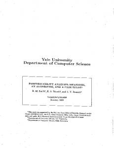
4.2 Implementing NoiseDown To describe an algorithm for sampling from the Noise Down distribution (Equation 6), it is sufficient to fix Y = y for some real constant y and fix parameters µ, λ, and λ# . Let f : R → [0, 1] be
y-1
y
y+1
y’ Figure 2: Illustration of f
defined by f (y# ) = fµ,λ,λ! (y # | Y = y), i.e., the conditional p.d.f. from Equation 6. We now describe an algorithm for sampling from the probability distribution defined by f . In the following derivation, we focus on the case where µ ≤ y; we will describe later the modifications that are necessary to handle the case where µ > y. Let ξ = min{µ, y − 1}. By Equation 6, for any y# ≤ ξ, f (y # ) = ey
!
/λ!
· γ(λ# , λ, y # , y) ·
) −µ λ y − µ* , · exp + # # λ λ λ
where 1 1 % & · 4λ cosh λ1! − 1 " # %1& % −y & % 1−y & % −1−y & · 2 cosh λ! · exp λ − exp λ − exp . λ
γ(λ# , λ, y # , y) = ey
!
/λ
·
(Note that the function γ above is as defined in Equation 7 but takes a simplified form given y# < ξ). As µ, y, λ, and λ# are all given, f (y # ) ∝ exp(y # /λ# + y # /λ) holds. Similarly, it can be verified that 1. ∀y # ∈ (ξ, y − 1], f (y # ) ∝ exp(y # /λ − y # /λ# ); 2. ∀y # ∈ [y + 1, +∞), f (y # ) ∝ exp(−y # /λ# − y # /λ). For example, Figure 2 illustrates f with the y-axis in log-scale. In summary, f conforms to an exponential distribution on each of the following intervals: (−∞, ξ], (ξ, y − 1], and [y + 1, +∞). When the probability mass of f on each of the three intervals is known, it is straightforward to generate random variables that +ξ follow f on those intervals. Let θ1 = −∞ f (y # )dy # , θ2 = + y−1 + +∞ f (y # )dy # , and θ3 = y+1 f (y # )dy # . It can be shown that ξ % & % & λ· cosh( λ1! ) − cosh( λ1 ) · exp ( λ1! + λ1 )·(ξ − µ) % & , (8) 2(λ# + λ) · cosh( λ1! ) − 1 * ) ! ! λ · cosh( λ1! ) · e1/λ − e1/λ · (1 − e−1/λ −1/λ ) % & θ2 = 4(λ − λ# ) · cosh( λ1! ) − 1 " ) 1 *# 1 · 1 − exp ( # − ) · (ξ − y + 1) , (9) λ λ % & % & λ · cosh( λ1! ) − cosh( λ1 ) · exp µ−y−1 − µ−y+1 λ! λ % & . (10) θ3 = 2(λ# + λ) · cosh( λ1! ) − 1 θ1 =
For the remaining interval (y − 1, y + 1) on which f has a complex form, we resort to a standard importance sampling approach. Specifically, we first generate a random sample y# that is uniformly distributed in (y − 1, y + 1). After that, we toss a coin that comes
Algorithm NoiseDown (µ, y, λ, λ# ) 1. initialize a boolean variable invert = true 2. if µ > y 3. set µ = −µ, y = −y, and invert = false 4. ξ = min{µ, y − 1} 5. let θ1 , θ2 , θ3 , and ϕ be as defined in Eqn. 8, 9, 10, and 11 6. generate a random variable u uniformly distributed in [0, 1] 7. if u ∈ [0, θ1 ) 8. generate a random variable y# ∈ (−∞, ξ] such that P r[y # = y # ] ∝ exp(y # /λ# + y # /λ) 9. else if u ∈ [θ1 , θ1 + θ2 ] 10. generate a random variable y# ∈ (ξ, y − 1] such that P r[y # = y # ] ∝ exp(y # /λ − y # /λ# ) 11. else if u ∈ [1 − θ3 , 1] 12. generate a random variable y# ∈ [y + 1, +∞) such that P r[y # = y # ] ∝ exp(−y # /λ# − y # /λ) 13. else 14. while true 15. generate a random variable y# uniformly distributed in (y − 1, y + 1) 16. generate a random variable u# uniformly distributed in [0, 1] 17. if u# ≤ f (y # )/ϕ then break 18. if invert = true then return y# ; otherwise, return −y#
Algorithm iReduct (T , Q, δ, $, λmax , λ∆ ) 1. let m = |Q| and qi be the i-th (i ∈ [1, m]) query in Q 2. initialize Λ = [λ1 , . . . , λm ], such that λi = λmax 3. if GS(Q, Λ) > $ then return ∅ 4. Y = LaplaceNoise(T, Q, Λ) 5. let Q# = Q 6. while Q# '= ∅ 7. Q∆ = PickQueries(Q# , Y, Λ, δ) 8. for each i ∈ [1, m] 9. if qi ∈ Q∆ then λi = λi − λ∆ 10. if GS(Q, Λ) ≤ $ 11. for each i ∈ [1, m] ! " 12. if qi ∈ Q∆ then yi = NoiseDown qi (T ), yi , λi + λ∆ , λi 13. else 14. for each i ∈ [1, m] 15. if qi ∈ Q∆ then λi = λi + λ∆ 16. Q# = Q# \ Q∆ 17. return Y
Figure 4: The iReduct Algorithm
Figure 3: The NoiseDown Algorithm up heads with a probability f (y# )/ϕ, where %1& % 1& 1 cosh λ! − exp − λ % & ϕ= # · 2λ cosh λ1! − 1 " # y−µ max{0, y − µ − 1} · exp − . λ λ#
(11)
If the coin shows a tail, we resample y# from a uniform distribution on (y − 1, y + 1), and we toss the coin again. This process is repeated until the coin shows a head, at which time we return y# as a sample from f . The following proposition proves the correctness of our sampling approach. P ROPOSITION 4 (N OISE D OWN S AMPLING ). Given µ ≤ y, we have f (y# ) < ϕ for any y# ∈ (y − 1, y + 1). ! So far, we have focused on the case where µ ≤ y. For the case when µ > y, we first set µ = −µ, y = −y, and then generate y # using the method described above. After that, we set y# = −y # before returning it as a sample from f . The correctness of this method follows from the following property of the Noise Down distribution fµ,λ,λ! (y # |Y = y) (as defined Equation 6): fµ,λ,λ! (y # |Y = y) = f−µ,λ,λ! (−y # |Y = −y)
for any µ, λ, λ# , y # , y. As a summary, Figure 3 shows the pseudocode of the NoiseDown function that takes as input µ, y, λ, λ# and returns a sample from the distribution defined in Equation 6.
4.3 The iReduct Algorithm We are now ready to present the iReduct algorithm, as illustrated in Figure 4. It takes as input a dataset T , a sequence Q of queries on T , a sanity bound δ, and three positive real numbers !, λmax , and λ∆ . iReduct starts by initializing a variable λi for each query qi ∈ Q (i ∈ [1, m]), setting λi = λmax (Lines 1-2). The userspecified parameter λmax is a large constant that corresponds to the greatest amount of Laplace noise that a user is willing to accept in any query answer returned by iReduct. For example, if Q is a sequence of count queries on T then a user may set λmax to 10% of the number of tuples in the dataset T .
As a second step, iReduct checks whether the conservative setting of the noise scale guarantees !-differential privacy (Line 3). This is done by measuring the generalized sensitivity of the query sequence given noise scales Λ. If the generalized sensitivity exceeds !, iReduct returns an empty set to indicate that the results of Q cannot be released without adding excessive amounts of noise to the queries. Otherwise, iReduct generates a noisy result yi for each query qi ∈ Q by applying Laplace noise of scale λi (Line 4). Given Y , iReduct iteratively applies NoiseDown to adjust the noise in yi so that noise magnitude is reduced for queries that appear to have high relative errors (Lines 5-16). In each iteration, iReduct first identifies a set Q∆ of queries (Line 7) and then tries to decrease the noise scales of the queries in Q∆ by a constant λ∆ (Lines 8-16). The selection of Q∆ is performed by an applicationspecific function that we refer to as PickQueries. An instantiation of PickQueries is given in Section 5.3, but in general, any algorithm can be applied, so long as the algorithm utilizes only the sanity bound δ, the noisy queries answers seen so far, and the queries’ noise scales, and does not rely on the true answer qi (T ) of any query qi . This requirement ensures that the selection of Q∆ does not reveal any private information beyond what has been disclosed by the noisy results generated so far. For example, if we aim to minimize the maximum relative error of the query results, we may implement PickQueries as a function that returns the query qi that maximizes λi / max{yi , δ}, i.e., the query whose noise scale is likely to be large with respect to its actual result. Once Q∆ is selected and the scales λi have been adjusted accordingly, iReduct checks whether the revised scales are permissible given the privacy budget. This is done by measuring the generalized sensitivity given the revised scales (Line 10). If the revised scales are permissible, iReduct applies NoiseDown to reduce the noise scale of each qi in Q∆ by λ∆ (Lines 11-12). Otherwise, iReduct reverts the changes in Λ and removes the queries in Q∆ from its working set (Line 13-16). This iterative process is repeated until no more queries remain in the working set, which indicates that iReduct cannot find a subset of queries whose noise can be reduced without violating the privacy constraint. At this point, it outputs the noisy answers Y .
T HEOREM 2 (P RIVACY OF iReduct). iReduct ensures !# differential privacy whenever its input parameter ! satisfies ! ≤ !# . !
5.
CASE STUDY: PRIVATE MARGINALS
In this section, we present an instantiation of the TwoPhase and iReduct algorithms for generating privacy-preserving marginals. Section 5.1 describes the problem and discusses existing solutions and Sections 5.2 and 5.3 describe the instantiations of TwoPhase and iReduct.
5.1 Motivation and Existing Solution A marginal is a table of counts that summarize a dataset along some dimensions. Marginals are widely used by the U.S. Census Bureau and other federal agencies to release statistics about the U.S. population. More formally, a marginal M of a dataset T is a table of counts that corresponds to a subset A of the attributes in T . If A contains k attributes A1 , A2 , . . . , Ak , then M comprises , k i=1 |Ai | counts, where |Ai | denotes the number of values in the domain of Ai . Each count in M pertains to a point *v1 , v2 , . . . , vk + in the k-dimensional space A1 ×A2 ×· · ·×Ak , and the count equals the number of tuples whose value on Ai is vi (i ∈ [1, k]). For example, Table 2 illustrates a dataset T that contains three attributes: Age, (Marital) Status, and Gender. Table 3 shows a marginal of T on {Status, Gender}. In general, a marginal defined over a set of k attributes is referred to as a k-dimensional marginal. While a dataset with k attributes can be equivalently represented as a single k-dimensional marginal, such a marginal is likely very sparse (i.e., all counts near zero), and thus will not be able to tolerate the random noise added for privacy. Instead, we therefore publish a set M of low dimensional marginals, each of which is a projection onto j dimensions for some small j < k. This is common practice at statistical agencies, and is consistent with prior work on differentially private marginal release [1]. We can publish M in a !-differentially private manner as long as we add Laplace noise of scale 2 · |M|/! to each count in every marginal. This is because changing a record affects only two counts in each marginal (each count would be offset by one), thus the sensitivity of the marginals is 2·|M|, i.e., Laplace noise of scale 2 · |M|/! suffices for privacy, as shown in Proposition 1. However, adding an equal amount of noise to each marginal in M may lead to sub-optimal results. For example, suppose that M contains two marginals M1 and M2 , such that M1 (M2 ) has a large (small) number of counts, all of which are small (large). If identical amount of noise is injected to M1 and M2 , then the noisy counts in M1 would have much higher relative errors than the noisy counts in M2 . Intuitively, a better solution is to apply smaller (larger) amount of noise to M1 (M2 ), so as to balance the quality of M1 and M2 without degrading their overall privacy guarantee. We measure the utility of a set of noisy marginals in terms of minimizing overall error, as defined next. Each marginal Mi ∈ M is represented as a sequence of queries [qi1 , . . . , qi|Mi | ] where qij denotes the jth query in Mi for i ∈ [1, |M|] and j ∈ [1, |Mi |]. Let Mi∗ denote a noisy version of marginal Mi and let yij denote to the noisy answer to qij for i ∈ [1, |M|] and j ∈ [1, |Mi |]. D EFINITION 6 (OVERALL E RROR OF M ARGINALS ). The ∗ } is overall error of a set of noisy marginals {M1∗ , . . . , M|M| defined as ∗
!
|Mi | |M| ! ! |yij − qij (T )| 1 1 · · ∗ |M| i=1 |Mi | j=1 max{δ, qij (T )}
We next describe how we instantiate TwoPhase and iReduct with this utility goal in mind. The query sequence input to both algorithms is simply the concatenation of the
Age 23 25 35 37 85
Status Single Single Married Married Widowed
Gender M F F F F
Table 2: A dataset T
Status Single Married Divorced Widowed
Gender M F 1 1 0 2 0 0 0 1
Table 3: A marginal of T
individual query sequences for each marginal; i.e., Q [q11 , . . . , q1|M1 | , . . . , q|M|1 , . . . , q|M||M|M| | ].
=
5.2 Instantiation of TwoPhase To instantiate TwoPhase, we must describe the implementation of the Rescale subroutine that was treated as a “black box” in Section 3.2. Let us first consider an ideal scenario where the first phase of TwoPhase returns the exact count of every query qij . In this case, we know that if we added Laplace noise of scale λi to every count in a marginal Mi , then each count qij (T ) in Mi would have an expected relative error of λi / max{δ, qij (T )}. (Recall that the expected absolute deviation of a Laplace variable equals its scale.) The expected relative error &in Mi would there% $|Maverage i| fore be λi /|Mi | · j=1 1/ max{δ, qij (T )} . Consequently, to minimize the expected overall error of the marginals, it suffices to & $ i| $ % 1/ max{δ, q (T )} is miniensure that Mi λi /|Mi | · |M ij j=1 mized, subject to the privacy constraint that the marginals should $ ensure !-differential privacy, i.e., |M| i=1 2/λi ≤ !. Using a Lagrange it can be shown that λi should be proportional - multiplier, $ i| to |Mi |/( |M j=1 1/ max{δ, qij (T )}). We refer to this optimal strategy for deciding noise scale as the Oracle method. Oracle is similar to the Proportional algorithm described in Section 3.1, but sets its λi values to minimize average rather than worst-case relative error. Rescale sets the noise scale similarly to how it is set by Oracle except that it uses the noisy counts to approximate the exact counts. $ i| To be precise, λi is proportional to |Mi |/ |M j=1 max{δ, yij }, where yij denotes the noisy answer produced by the first phase of TwoPhase.
5.3 Instantiation of iReduct Before we can use iReduct to publish marginals, we need to instantiate two of its subroutines: (i) a method for computing the generalized sensitivity of a set of weighted marginal queries and (ii) an implementation of the PickQueries black box (discussed in Section 4.3) that chooses a set Q∆ of marginal queries for noise reduction. In practice, the sensitivity of a set of marginals depends only on the smallest noise scale in each marginal, and so we gain the best tradeoff between low sensitivity and high utility by always selecting the same noise scale for every count in a given marginal. We maintain the invariant by (i) initially setting all marginal counts to have the same noise scale λmax and (ii) having PickQueries always pass to NoiseDown the queries corresponding to a single marginal Mi∗ in which the noise scale for each cell in Mi∗ is reduced by the same constant λ∆ . As the counts in the same marginal always have identical noise scale, we can easily derive the generalized sensitivity of the marginal queries as follows. Assume that, in the beginning of a certain iteration, the counts in Mi∗ (i ∈ [1, |M|]) have noise scale λi .
Brazil US
Age 101 92
Gender 2 2
Marital Status 4 4
State 26 51
Birth Place 29 52
Race 5 14
Education 5 5
Occupation 512 477
Class of Worker 4 4
Table 4: Sizes of Attribute Domains It can be verified that the generalized sensitivity of the marginals is ! 2 (12) gα = λi i∈[1,|M|]
Consider that we apply NoiseDown on a noisy marginal Mj∗ (j ∈ [1, |M|]). The noise scale of the queries in Mj∗ would become λj − λ∆ , in which case the generalized sensitivity would become: ! 2 2 gβ = + . (13) λj − λ∆ λi
0.14 0.12 0.1 0.08 0.06 0.04 0.02 0
overall error TwoPhase
0 0.1 0.2 0.3 0.4 0.5 0.6 ε1 / ε
0.07 0.06 0.05 0.04 0.03 0.02 0.01 0
(a) Brazil
overall error TwoPhase
0 0.1 0.2 0.3 0.4 0.5 0.6 ε1 / ε (b) USA
i∈[1,|M|]∧i'=j
Recall that, in each iteration of iReduct, we aim to ensure that the generalized sensitivity of the queries does not exceed !. Therefore, we can apply NoiseDown on a marginal Mj∗ only if gβ ≤ !. We now discuss our implementation of the PickQueries function. Notice that when we apply NoiseDown to a noisy marginal Mj∗ (j ∈ [1, |M|]), the expected errors of the estimated counts for that marginal decrease (due to the decrease in the noise scale of Mj∗ ) but the privacy guarantee degrades. Ideally, running NoiseDown on the selected marginal should lead to a large drop in the overall error and a small increase in the privacy overhead. To identify good candidates, we adopt the following methods to quantify the changes in the overall error and privacy overhead that are incurred by invoking NoiseDown on a marginal Mj∗ . First, recall that when we employ NoiseDown to reduce the noise scale λj of Mj∗ by a constant λ∆ , the generalized sensitivity of the noisy marginals increases from gα to gβ , where gα and gβ are as defined in Equations 12 and 13. In light of this, we quantify the cost of privacy entailed by applying NoiseDown on Mj∗ as gβ − gα =
2 2 − . λj − λ∆ λj
(14)
Second, for each noisy count y in Mj∗ , we estimate its relative error as λj / max{y, δ}, where δ is the sanity bound. In other words, we use y to approximate the true count, and we estimate the absolute error of y as the expected absolute deviation λj of the Laplace noise added in y. Accordingly, the average relative error of Mj∗ $ is estimated as λj · y∈M ∗ 1/ max{y, δ}. Following the same j
rationale, we estimate the average relative$error of Mj∗ after the application of NoiseDown as (λj − λ∆ ) · y∈M ∗ 1/ max{y, δ}. j Naturally, the decrease in the overall error of the marginals (re∗ sulted from invoking NoiseDown on Mj ) is quantified as * ) ! ! 1 1 1 · λj · − (λj − λ∆ ) · |M| max{y, δ} max{y, δ} ∗ ∗ y∈Mj
=
λ∆ · |M|
y∈Mj
!
y∈Mj∗
1 max{y, δ}
(15)
Given Equations 14 and 15, in each iteration of iReduct, we heuristically choose the marginal Mj∗ that maximizes *.) )λ ! 2 1 2* ∆ . − · |M| max{y, δ} λj − λ∆ λj ∗ y∈Mj
That is, we select the marginal that maximizes the ratio between the estimated decrease in overall error and the estimated increase in privacy cost.
Figure 5: Overall Error vs. !1 /! (1D Marginals)
6. EXPERIMENTS We evaluate the accuracy of the proposed algorithms on three tasks: estimating all one-way marginals (Section 6.3), estimating all two-way marginals (Section 6.4), and learning a Naive Bayes classifier (Section 6.5).
6.1 Experimental Settings We use two datasets2 that are composed of census records collected from Brazil and the US respectively. Each dataset contains nine attributes, whose domain sizes are as illustrated in Table 4. The Brazil dataset consists of nearly 10 million tuples, while the US dataset has around 14 million records. We use iReduct to generate noisy marginals from each dataset, and we compare the performance of iReduct against four alternate methods. The first method is the Oracle algorithm presented in Section 5.2, which utilizes the exact counts in the marginals to decide the noise scale of each marginal in a manner that minimizes the expected overall error. Although Oracle does not conform to !differential privacy, it provides a lower bound on the error incurred by any member of a large class of !-differential privacy algorithms. The second and third methods are the TwoPhase and iResamp algorithms presented in Section 3 and Appendix A respectively. The final technique, henceforth referred to as Dwork, is Dwork et al.’s method (Section 2.2), which adds an equal amount of noise to each marginal. We measure the quality of noisy marginals by their overall errors, as defined in Section 5.1. In every experiment, we run each algorithm 10 times, and we report the mean of the overall errors incurred by the algorithm. Among the input parameters of iReduct, we fix λmax = |T |/10 and λ∆ = |T |/106 , where |T | denotes the number of tuples in the dataset. That is, iReduct starts by adding Laplace noise of scale |T |/10 to each marginal and, in each iteration, it reduces the noise scale of a selected marginal by |T |/106 . All of our experiments are run on a computer with a 2.66GHz CPU and 24GB memory.
6.2 Calibrating TwoPhase As was discussed in Section 3.2, the performance of the TwoPhase algorithm depends on how the fixed privacy budget is allocated across its two phases. This means that before we can use 2 Both datasets are available online as part of the Integrated Public Use Microdata Series [25].
iReduct
1
Oracle
TwoPhase
overall error
1
iReduct
Dwork
0.1
0.1 0.2
iResamp
overall error
0.4 0.6 0.8 1 ε (×10-2) (a) Brazil
0.2
0.4 0.6 0.8 1 ε (×10-2) (b) USA
Figure 6: Overall Error vs. ! (1D Marginals) iReduct
Oracle
overall error 0.25 0.2 0.15 0.1 0.05 0 0.2 0.4 0.6 0.8 -4 δ / |T| (×10 ) (a) Brazil
TwoPhase
1
iResamp
Oracle
overall error 1.6 1.4 1.2 1 0.8 0.6 0.4 0.2 0 0.2 0.4 0.6 0.8 ε (×10-2) (a) Brazil
TwoPhase
1
iResamp
Dwork
overall error 1.2 1 0.8 0.6 0.4 0.2 0 0.2 0.4 0.6 0.8 ε (×10-2) (b) USA
1
Figure 8: Overall Error vs. ! (2D Marginals) Dwork
overall error 0.09 0.08 0.07 0.06 0.05 0.04 0.03 0.02 0.01 0 0.2 0.4 0.6 0.8 -4 δ / |T| (×10 ) (b) USA
iReduct
Oracle
TwoPhase
overall error
1
Figure 7: Overall Error vs. δ (1D Marginals) the TwoPhase algorithm, we must decide how to set the values of !1 and !2 to optimize the quality of the noisy marginals. To determine the appropriate setting, we fix ! = 0.01 and measure the overall error of TwoPhase when !1 varies and !2 = ! − !1 . Figure 5 illustrates the overall error on the set of one-dimensional marginals as a function of !1 /!. As !1 /! increases, the overall error of TwoPhase decreases until it reaches a minimum and then increases monotonically. When !1 is too small, the first step of TwoPhase is unable to generate accurate estimates of the marginal counts. This renders the second step of TwoPhase less effective, since it relies on the estimates from the first step to determine the noise scale for each marginal. On the other hand, making !1 too large causes !2 to becomes small and forces the second step to inject large amounts of noise into all of the marginal counts. The utility of the noisy marginals is optimized only when !1 /! strikes a good balance between the effectiveness of the first and second steps. As shown in Figure 5, the overall error of TwoPhase hits a sweet spot when !1 ∈ [0.06!, 0.08!]. We set !1 = 0.07! in the experiments that follow.
6.3 Results on 1D Marginals We compare the overall error incurred when each of the five algorithms described above is used to produce differentially private estimates of the one-dimensional marginals of the Brazil and USA census data. We vary both ! and δ. Figure 6 shows the overall error of each algorithm as a function of !, with δ fixed to 10−4 · |T |. iReduct yields error values that are almost equal to those of Oracle, which indicates that its performance is close to optimal. TwoPhase performs worse than iReduct in all cases, but it still consistently outperforms the other methods. The overall error of iResamp is comparable to that of Dwork. Figure 7 illustrates the overall error of each method as a function of the sanity bound δ when ! = 0.01. The relative performance of each method is the same as in Figure 6. The overall errors of all algorithms decrease as δ increases, since a larger δ leads to lower relative errors for marginal counts smaller than δ (see Equation 1).
1.2 1 0.8 0.6 0.4 0.2 0 0.2
0.4 0.6 0.8 -4 δ / |T| (×10 ) (a) Brazil
iResamp
Dwork
overall error
1
0.8 0.7 0.6 0.5 0.4 0.3 0.2 0.1 0 0.2
0.4 0.6 0.8 -4 δ / |T| (×10 ) (b) USA
1
Figure 9: Overall Error vs. δ (2D Marginals)
In the aforementioned experiments, every method but iReduct needs only a few linear scans of the marginal counts to generate its output, and therefore incurs negligible computation cost. In contrast, the inner loop of iReduct is executed O(λmax /λ∆ ) times, and the iReduct takes around 5 seconds to output a set of marginal counts. The relative high computational overhead of iReduct is justified by the fact that it provides improved data utility over the other methods.
6.4 Results on 2D Marginals In the second sets of experiments, we consider the task of generating all two-dimensional marginals of the datasets. For the input parameters of TwoPhase, we set !1 /! = 0.025 based on an experiment similar to that described in Section 6.2. Figure 8 shows the overall error of each method when δ = 10−4 · |T | and ! varies. The overall error of iReduct is almost the same as that of Oracle. TwoPhase is outperformed by iReduct, but its overall error is consistently lower than that of iResamp or Dwork. Interestingly, the performance gaps among iReduct, TwoPhase, and Dwork are not as substantial as the case for one-dimensional marginals. The reason is that a large fraction of the two-dimensional marginals are sparse. As a consequence, iReduct and TwoPhase apply roughly equal amounts of noise to those marginals in order to reduce overall error. The noise scale of the marginals is therefore relatively uniform: the allocation of noise scale selected by iReduct or TwoPhase does not differ too much from the allocation used by Dwork. This explains why the improvement of iReduct and TwoPhase over Dwork is less significant. Figure 9 illustrates the overall error of each algorithm as a function of δ, with ! = 0.1. The relative performance of each technique remains the same as in Figure 8. Regarding computation cost, iReduct requires around 15 minutes to generate each set of two-dimensional marginals. This running time is considerably longer than for one-dimensional marginals because iReduct must handle more marginal counts in the twodimensional case.
iReduct
Oracle
overall error 6 5 4 3 2 1 0 0.1 0.2 0.4 ε (×10-2) (a) Brazil
0.7
TwoPhase
1
iResamp
overall error 3.5 3 2.5 2 1.5 1 0.5 0 0.1 0.2 0.4 ε (×10-2) (b) USA
Dwork
0.7 1
Figure 10: Overall Error vs. ! (Marginals for Classifier)
0.74 0.72 0.7 0.68 0.66 0.64
Noise-Free
iReduct
Two-Phase
iResamp
overall error
0.1
0.2 0.4 ε (×10-2) (a) Brazil
Oracle Dwork
overall error
0.7 1
0.74 0.72 0.7 0.68 0.66 0.64 0.62 0.6 0.1
0.2 0.4 ε (×10-2) (b) USA
0.7 1
Figure 11: Accuracy of Classifier vs. !
6.5 Results on Naive Bayes Classifier Our last set of experiments demonstrates that relative error is an important metric for real-world analytic tasks. In these experiments, we consider the task of constructing a Naive Bayes classifier from each dataset. We use Education as the class variable and the remaining attributes as feature variables. The construction of such a classifier requires 9 marginals: a one-dimensional marginal on Education and 8 two-dimensional marginals, each of which contains Education along with another attribute. We apply each algorithm to generate noisy versions of the 9 marginals, and we measure the accuracy of the classifier built from the noisy data3 . For robustness of measurements, we adopt 10-fold crossvalidation in evaluating the accuracy of classification. That is, we first randomly divide the dataset into 10 equal-size subsets. Next, we take the union of 9 subsets as the training set and use the remaining subset for validation. This process is repeated 10 times in total, using each subset for validation exactly once. We report (i) the average overall error of the 10 sets of noisy marginals generated from the 10 training datasets and (ii) the average accuracy of the classifiers built from the 10 sets of noisy marginals. Figure 10 illustrates the overall error incurred by each algorithm when δ = 10−4 · |T | and ! varies. (The input parameter !1 of TwoPhase is set to 0.03 based on an experiment similar to that described in Section 6.2.) Again, iReduct and Oracle entail the smallest errors in all cases, followed by TwoPhase. In addition, iResamp consistently incurs higher error than Dwork does. Figure 11 shows the accuracy of the classifiers built upon the output of each algorithm. The dashed line in the figure illustrates the accuracy of a classifier constructed from a set of marginals without any injected noise. Observe that methods that incur lower relative errors lead to more accurate classifiers.
7.
RELATED WORK
There is a plethora of techniques [1–5, 5, 9–12, 14, 15, 17–20, 22, 26–28, 32] for enforcing !-differential privacy in the publication of various types of data, such as relational tables [9,17,21,32], search logs [15, 20], data mining results [12, 23], and so on. None of these techniques optimizes the relative errors of the published data; instead, they optimize either (i) the variance of the noisy results or (ii) some application-specific metric such as the accuracy of classification [12]. Below, we will discuss several pieces of work that are closely related to (but different from) ours. Barak et al. [1] devise a technique for publishing marginals of a given dataset. Their objective, however, is not to improve the accuracy of the released marginal counts. Instead, their technique is de3
Following previous work [6], we postprocess each noisy marginal cell y by setting y = max{y + 1, 1} before constructing the classifier from the marginals.
signed to make the noisy marginals more user-friendly by ensuring that (i) every marginal count is non-negative and (ii) all marginals are consistent, i.e. the sum of the counts in one marginal should equal the sum in any other marginal. Kasiviswanathan et al. [19] present a theoretical study on marginal publishing, and they prove several lower bounds on the absolute errors of the noisy marginal counts. Nevertheless, they do not propose any concrete algorithm for releasing marginals. Blum et al. [4] present a method for releasing one-dimensional data that provides a worst-case guarantee on the absolute errors of range count query results. Hay et al. [17] propose a algorithm that improves the performance bound of Blum et al.’s method, while Xiao et al. [32] devise an approach for multi-dimensional data that achieves a bound similar to Hay et al.’s. Li et al. [21] generalize both Hay et al.’s and Xiao et al.’s approaches, and propose an optimal technique that minimizes the absolute errors of any given set of range count queries. In principle, the techniques above can also be adapted for marginal publishing, since each marginal count can be regarded as the answer to a range count query. However, since those techniques optimize only the absolute errors of the marginal counts, they would incur large relative errors for small counts in the marginals, as is the case for Dwork et al’s method. Besides the aforementioned work on !-differential privacy, there is also a technique by Xiao et al. [31] that is worth mentioning. Given a dataset T , Xiao et al.’s technique generates a collection ∗ of noisy datasets {T1∗ , T2∗ , . . . , Tm } that satisfies two conditions. ∗ First, for any j < i, Tj contains more noise than Ti∗ . Second, ∗ ∗ P r[T | T1∗ , . . . , Tm ] = P r[T | Tm ], i.e., the combination of all noisy data reveals no more information than the least noisy ver∗ of T . Our NoiseDown algorithm provides a very similar sion Tm guarantee. Nevertheless, Xiao et al.’s method cannot be used to implement NoiseDown, since their method is applicable only when the noisy data is computed using an approach called randomized response [30]. In contrast, NoiseDown requires that the the noise injected into query outputs follow a Laplace distribution.
8. CONCLUSIONS Existing techniques for differentially private query publishing optimize only the absolute error of the published query results, which may lead to large relative errors for queries with small answers. This paper remedies the problem with iReduct, a novel algorithm for generating differentially private results with reduced relative errors. We present an instantiation of iReduct for generating marginals, and we demonstrate its effectiveness through extensive experiments with real data. iReduct outperforms several other candidate approaches and, unlike TwoPhase, it does not require parameter tuning. Our technique for generating marginals could be used as a ba-
sis for releasing a table of “synthetic” records. Since our computations are differentially private, the table would satisfy a much stronger guarantee than approaches based on anonymity. Furthermore, many counting queries executed on the synthetic records would have low relative errors relative to the original data. There is a tight connection between marginals and log-linear statistical models, as well as algorithms for sampling [7]. However, a challenge remains: the noise introduced for privacy may produce marginals that are infeasible, meaning that it is impossible to construct a table that is consistent with the marginals. Finally, note that the iReduct algorithm introduces subtle correlations between the answers that it outputs. This is because the magnitude of the noise injected into each query answer depends not only on the true answer for that query but also on noisy answers to the other queries under consideration. We believe that such correlations may be necessary to minimize relative error. In fact, differentially private techniques that produce correlated answers are not uncommon [1, 4, 15, 17, 21, 29]. Further investigation into the implications of such correlations is left as future work.
9.
ACKNOWLEDGMENTS
This work was supported by Nanyang Technological University under SUG Grant M58020016 and AcRF Tier 1 Grant RG 35/09, by the Agency for Science, Technology and Research (Singapore) under SERG Grant 1021580074, by the Computing Innovation Fellows Project (http://cifellows.org/), funded by the Computing Research Association/Computing Community Consortium through NSF Grant 1019343, by the NSF under Grants IIS-0627680 and IIS-1012593, and by the New York State Foundation for Science, Technology, and Innovation under Agreement C050061. Any opinions, findings, conclusions or recommendations expressed are those of the authors and do not necessarily reflect the views of the sponsors.
10. REFERENCES [1] B. Barak, K. Chaudhuri, C. Dwork, S. Kale, F. McSherry, and K. Talwar. Privacy, accuracy, and consistency too: a holistic solution to contingency table release. In Proc. of ACM Symposium on Principles of Database Systems (PODS), pages 273–282, 2007. [2] A. Beimel, S. P. Kasiviswanathan, and K. Nissim. Bounds on the sample complexity for private learning and private data release. In Theory of Cryptography Conference (TCC), pages 437–454, 2010. [3] R. Bhaskar, S. Laxman, A. Smith, and A. Thakurta. Discovering frequent patterns in sensitive data. In Proc. of ACM Knowledge Discovery and Data Mining (SIGKDD), pages 503–512, 2010. [4] A. Blum, K. Ligett, and A. Roth. A learning theory approach to non-interactive database privacy. In Proc. of ACM Symposium on Theory of Computing (STOC), pages 609–618, 2008. [5] K. Chaudhuri and C. Monteleoni. Privacy-preserving logistic regression. In Proc. of the Neural Information Processing Systems (NIPS), pages 289–296, 2008. [6] G. Cormode. Individual privacy vs population privacy: Learning to attack anonymization. Computing Research Repository (CoRR), abs/1011.2511, 2010. [7] P. Diaconis and B. Sturmfels. Algebraic algorithms for sampling from conditional distributions. Annals of Statistics, 1998.
[8] C. Dwork. Differential privacy. In International Colloquium on Automata, Languages and Programming (ICALP), pages 1–12, 2006. [9] C. Dwork, F. McSherry, K. Nissim, and A. Smith. Calibrating noise to sensitivity in private data analysis. In Theory of Cryptography Conference (TCC), pages 265–284, 2006. [10] C. Dwork, M. Naor, T. Pitassi, and G. N. Rothblum. Differential privacy under continual observation. In Proc. of ACM Symposium on Theory of Computing (STOC), pages 715–724, 2010. [11] D. Feldman, A. Fiat, H. Kaplan, and K. Nissim. Private coresets. In Proc. of ACM Symposium on Theory of Computing (STOC), pages 361–370, 2009. [12] A. Friedman and A. Schuster. Data mining with differential privacy. In Proc. of ACM Knowledge Discovery and Data Mining (SIGKDD), pages 493–502, 2010. [13] M. N. Garofalakis and A. Kumar. Wavelet synopses for general error metrics. ACM Transactions on Database Systems (TODS), 30(4):888–928, 2005. [14] A. Ghosh, T. Roughgarden, and M. Sundararajan. Universally utility-maximizing privacy mechanisms. In Proc. of ACM Symposium on Theory of Computing (STOC), pages 351–360, 2009. [15] M. Götz, A. Machanavajjhala, G. Wang, X. Xiao, and J. Gehrke. Publishing search logs - a comparative study of privacy guarantees. IEEE Transactions on Knowledge and Data Engineering (TKDE), 99, 2011. [16] M. Hardt and K. Talwar. On the geometry of differential privacy. In Proc. of ACM Symposium on Theory of Computing (STOC), 2010. [17] M. Hay, V. Rastogi, G. Miklau, and D. Suciu. Boosting the accuracy of differentially private histograms through consistency. Proc. of Very Large Data Bases (VLDB) Endowment, 3(1):1021–1032, 2010. [18] S. P. Kasiviswanathan, H. K. Lee, K. Nissim, S. Raskhodnikova, and A. Smith. What can we learn privately? In Symposium on Foundations of Computer Science (FOCS), pages 531–540, 2008. [19] S. P. Kasiviswanathan, M. Rudelson, A. Smith, and J. Ullman. The price of privately releasing contingency tables and the spectra of random matrices with correlated rows. In Proc. of ACM Symposium on Theory of Computing (STOC), pages 775–784, 2010. [20] A. Korolova, K. Kenthapadi, N. Mishra, and A. Ntoulas. Releasing search queries and clicks privately. In International World Wide Web Conference (WWW), pages 171–180, 2009. [21] C. Li, M. Hay, V. Rastogi, G. Miklau, and A. McGregor. Optimizing linear counting queries under differential privacy. In Proc. of ACM Symposium on Principles of Database Systems (PODS), pages 123–134, 2010. [22] A. Machanavajjhala, D. Kifer, J. M. Abowd, J. Gehrke, and L. Vilhuber. Privacy: Theory meets practice on the map. In Proc. of International Conference on Data Engineering (ICDE), pages 277–286, 2008. [23] F. McSherry and I. Mironov. Differentially private recommender systems: Building privacy into the netflix prize contenders. In Proc. of ACM Knowledge Discovery and Data Mining (SIGKDD), pages 627–636, 2009. [24] F. McSherry and K. Talwar. Mechanism design via
[25]
[26]
[27]
[28]
[29]
[30]
[31]
[32]
differential privacy. In Symposium on Foundations of Computer Science (FOCS), pages 94–103, 2007. Minnesota Population Center. Integrated public use microdata series – international: Version 5.0. 2009. https://international.ipums.org. K. Nissim, S. Raskhodnikova, and A. Smith. Smooth sensitivity and sampling in private data analysis. In Proc. of ACM Symposium on Theory of Computing (STOC), pages 75–84, 2007. V. Rastogi and S. Nath. Differentially private aggregation of distributed time-series with transformation and encryption. In Proc. of ACM Management of Data (SIGMOD), pages 735–746, 2010. A. Roth and T. Roughgarden. Interactive privacy via the median mechanism. In Proc. of ACM Symposium on Theory of Computing (STOC), pages 765–774, 2010. J. S. Vitter and M. Wang. Approximate computation of multidimensional aggregates of sparse data using wavelets. In Proc. of ACM Management of Data (SIGMOD), pages 193–204, 1999. S. L. Warner. Randomized response: A survey technique for eliminating evasive answer bias. J. of the American Statistical Association, 60(309):63–69, 1965. X. Xiao, Y. Tao, and M. Chen. Optimal random perturbation at multiple privacy levels. Proc. of Very Large Data Bases (VLDB) Endowment, 2(1):814–825, 2009. X. Xiao, G. Wang, and J. Gehrke. Differential privacy via wavelet transforms. In Proc. of International Conference on Data Engineering (ICDE), pages 225–236, 2010.
APPENDIX A.
ALTERNATE METHOD FOR NOISE REDUCTION
Let qi be a query, and let yi# (resp. yi ) be a noisy version of qi (T ) injected with Laplace noise of scale λ#i (resp. λi ), such that (i) λ#i < λi , and (ii) yi# and yi are generated independently. As discussed in Section 3, we can combine yi# and yi to obtain an estimate of qi (T ) that is more accurate than either yi# or yi alone. In particular, let #2 2 ∗ yi∗ = (λ2i · yi# + λ#2 i · yi )/(λi + λi ). It can be verified that yi has #2 2 #2 2 a variance 2λi λi /(λi + λi ), which is smaller than the variances of both yi# and yi . Furthermore, the variance of yi∗ is the minimum among all unbiased estimators of q(T ) given yi# and yi . Nevertheless, generating yi∗ is not cost-effective since, intuitively, it incurs a privacy overhead of 1/λ#i + 1/λi (i.e., the combined cost of producing yi# and yi ). In contrast, with the same privacy cost, we could have first generated yi and then applied NoiseDown on yi to obtain a noisy version of qi (T ) with a vari2 # 2 ∗ ance 2λ#2 i λi /(λi + λi ) , which is smaller than the variance of yi . This indicates that generating and combining independent noisy versions leads to lower data utility than NoiseDown does. To further illustrate this point, we present iResamp (iterative resampling), an alternative to iReduct that iteratively samples independent noisy query answers instead of using NoiseDown. We compare the performance of iResamp with that of iReduct in the experiments in Section 6. Figure 12 shows the pseudo-code of iResamp. Like iReduct, iResamp generates initial estimates of query values by adding a large amount of Laplace noise to the true values (Lines 1-5 in Figure 12) and then iteratively refines the noisy query results (Lines 6-21). In each iteration, it also invokes the PickQueries black box function to select a set Q∆ queries for noise reduction. The reduction pro-
Algorithm iResamp (T , Q, δ, $, λmax ) 1. let m = |Q| and qi be the i-th (i ∈ [1, m]) query in Q 2. initialize Λ = [λ1 , . . . , λm ], such that λi = λmax 3. if GS(Q, Λ) > $ then return ∅ 4. Y = LaplaceNoise(T, Q, Λ) 5. let Q# = Q 6. while Q# '= ∅ 7. Q∆ = PickQueries(Q# , Y, Λ, δ) 8. for each i ∈ [1, m] 9. if qi ∈ Q∆ then λi = λi /2 10. let Λ# = [λ#1 , . . . , λ#m ], such that λ#i = 1/(2/λi − 1/λmax ) 11. if GS(Q, Λ# ) ≤ $ 12. for each i ∈ [1, m] 13. if qi ∈ Q∆ (1) (k−1) 14. let yi , . . . yi be the noisy versions of qi (T ) that have been generated in the previous iterations (k) 15. yi = LaplaceNoise(T, qi , λi ) (1) (k) 16. calculate yi∗ based on yi , . . . yi according to Eqn. 16 ∗ 17. yi = yi 18. else 19. for each i ∈ [1, m] 20. if qi ∈ Q∆ then λi = 2λi 21. Q# = Q# \ Q∆ 22. return Y
Figure 12: The iResamp Algorithm cess, however, is not performed by applying NoiseDown, but by generating new noisy answers that are independent of the noisy estimates obtained in previous iterations (Line 15). Specifically, if the most recent noisy answer generated for a query qi ∈ Q∆ has noise scale λi then the new noisy result will have noise scale λi /2, i.e. the amount of noise is reduced by half each time a value is resampled (Lines 8-9). After the new noisy estimate is generated, iResamp takes a weighted average of all the noisy results that have been obtained for qi so far (Line 16) in order to derive a varianceminimized estimate of qi (T ). In particular, if there are k indepen(j) (j) dent noisy samples yi (j ∈ [1, n]) of qi (T ) such that yi has (j) noise scale λi , then the variance-minimized unbiased estimate of qi (T ) is: * ) $k (j) (j) (j) · λi j=1 yi / λi ∗ * . ) (16) yi = $ (j) (j) k 1/ λ · λ i i j=1 The new estimates are then used by the PickQueries function for query selections in the next iteration (Line 17). To show that the algorithm guarantees !-differential privacy, it suffices to show that the set of all noisy query estimates (generated in all iterations) of all the marginals is !-differentially private. No(k) tice that for any query qi , the k-th noisy answer yi for qi (generated by iResamp) has noise scale λmax /2k−1 . This is true because (1) the first noisy answer yi has noise scale λmax and the noise scale (j) (j−1) (j > 1). By sumof yi equals half of the noise scale of yi ming the terms of the resulting geometric series, it can be verified (1) (k) that the privacy cost of producing yi , . . . , yi is bounded above by the cost of generating a noisy answer for qi with Laplace noise (k) of scale 2/λi − 1/λmax , where λi denotes the noise scale of yi . Therefore, to ensure that all noisy results produced by iResamp are !-differentially private, it suffices to guarantee that the sequence Q of input queries has generalized sensitivity at most ! with respect to Λ# = [λ#1 , . . . , λ#m ], where λ#i = 1/(2/λi − 1/λmax ). This explains the rationale of Lines 10 and 11 in Figure 12. The above argument concludes our proof of the following theorem: T HEOREM 3 (P RIVACY OF iResamp). iResamp ensures !# differential privacy whenever its input parameter ! satisfies ! ≤ !# . !