R.L. Snyder, University of California, Land, Air and Water Resources, Davis, CA. M. Orang, California Department of Water Resources, Div. of Planning, ...
BASIC IRRIGATION SCHEDULING (BIS) R.L. Snyder, University of California, Land, Air and Water Resources, Davis, CA M. Orang, California Department of Water Resources, Div. of Planning, Sacramento, CA K. Bali, University of California, Cooperative Extension, Imperial County, Holtville, CA S. Eching, California Department of Water Resources, Office of Efficient Water Use, Sacramento, CA Copyright © 2000. Regents of the University of California, All rights reserved. Originally written - December 2000 Revised – April 2007
Introduction The Basic Irrigation Scheduling (BIS) application was written using MS Excel to help people plan irrigation management of crops. The BIS program can be downloaded by clicking on BIS.pdf BISe.xls BISm.xls
BIS Manual in English BIS Application Program (English units) BIS Application Program (metric units)
BISms.pdf BISms.xls
BIS Manual en Español BIS Programa en Español (sistema métrico)
BIS estimates annual trends of ETo using daily mean climate data by month, and it contains the most up-todate crop coefficient information available in California. The BIS application aids with the calculation of daily crop coefficient (Kc) values and crop Evapotranspiration (ETc), it helps to identify yield thresholds and management allowable depletions, and it provides a check book approach for determining irrigation timing and amount.
ETo Calculations In the worksheet “Weather”, either daily mean ETo rates or weather data are input to estimate ETo rates. Then BIS application uses a smooth curve fitting technique to estimate daily ETo rates during the year from the monthly data. Weather inputs can include the daily mean (1) solar radiation (MJ m-2 d-1), air temperature (oC), wind speed (m s-1), and dew point temperature (oC). In California, the monthly weather data can be extracted from the “California Climate Data.xls” program, which is available from the California Department of Water Resources from http://www.waterplan.water.ca.gov/landwateruse/wateruse/Ag/CUP/California_Climate_Data_010804.xls.
The BIS application calculates ETo using the Penman-Monteith (PM) equation (Monteith, 1965) as presented in the United Nations FAO Irrigation and Drainage Paper (FAO 56) by Allen et al. (1998) and using the Hargreaves-Samani (HS) equation (1982 and 1985). If only temperature data are input, but Hargreaves-Samani equation is used. For the ETo calculations, the station latitude and elevation must also be input. If the cells are left blank, then latitude 0o and elevation 0 meters above sea level are used. After calculating daily means by month, a cubic spline curve fitting subroutine is used to estimate daily ETo rates for the entire year. The estimated daily ETo values are automatically copied to the “Crop” worksheet and to the “MakeSchedule” worksheet in the column labeled “Average ETo”. Note that, if ETo data are available, they can be input directly into the Weather worksheet. However, the number of rainy days per month should also be input to properly determine crop coefficient (Kc) values. Pan evaporation data can also be
1
entered into the “Weather” worksheet under the column labeled “Ep” to estimate monthly ETo. To calculate ETo from pan evaporation data, the fetch (i.e., distance of grass around the pan) must also be input in the cell at the top of the Ep column. If both weather and ETo data are entered, the ETo entries will take precedence over the calculations from weather data. If all of the weather data are input, the PM estimate of ETo is used. If only temperature data are input, the PM ETo cannot be calculated and the HS equation is used. Explanations of how to calculate monthly average ETo using the Penman-Monteith and HargreavesSamani equations are described in documents available from the UCD biometeorology web page http://biomet.ucdavis.edu and in the FAO Irrigation and Drainage Paper 56 (Allen et al., 1998), which can be accessed using a link from the UCD biometeorology web page. Bare soil evaporation is estimated for each day of the year using daily ETo estimates and the numberof-rainy-days per month (NRD), which are input into the “Weather” worksheet. The NRD is used to estimate the days between rainfall for each month and the results are used with ETo to estimate bare soil evaporation (Es) using a 2-stage model. Then the estimated soil evaporation (Es) is used to calculate a daily mean Ke = Es/ETo value for bare soil for each month. Curve fitting is used to estimate daily values of Ke over the year. The Ke is a baseline coefficient, so the Kl values must be greater than or equal to Ke.
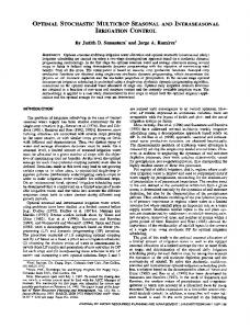
Crop Evapotranspiration ETc Calculation While reference crop evapotranspiration accounts for variations in weather and offers a measure of the "evaporative demand" of the atmosphere, crop coefficients account for the difference between the crop evapotranspiration (ETc) and ETo. The main factors affecting the difference between ETc and ETo are (1) light absorption by the canopy, (2) canopy roughness, which affects turbulence, (3) crop physiology, (4) leaf age, and (5) surface wetness. Because evapotranspiration (ET) is the sum of evaporation (E) from soil and plant surfaces and transpiration (T), which is vaporization that occurs inside of the plant leaves, it is often best to consider the two components separately. When not limited by water availability, ET is limited by the availability of energy to vaporize water. Therefore, solar radiation (or light) interception by the foliage and soil have a big effect on the ET rate. As a crop canopy develops, the ratio of T to ET increases until most of the ET comes from T and E is a minor component. This occurs because the light interception by the foliage increases until most light is intercepted before it reaches the soil. Therefore, crop coefficients for field and row crops generally increase until the canopy ground cover reaches about 75% and the light interception is near 80%. For tree and vine crops the peak Kc is reached when the canopy has reached about 63% ground cover. The difference between the crop types results because the light interception is greater for the taller crops. Bare Soil Kc Values During the off season and early during crop growth, E is the main component of ET. Therefore, a good estimate of the Kc for bare soil is useful to estimate off-season soil evaporation and ETc early in the season. A two-stage method for estimating soil evaporation presented by Stroonsnjider (1987) is used to estimate bare soil crop coefficients. In stage 1, the soil evaporation rate is limited by only by energy availability to vaporize water. In stage 2, the soil has dried sufficiently that soil hydraulic properties limit the transfer of water to the surface for vaporization. Figure 1 shows the bare soil Kc as a function of ETo rate and a range of soil wetting frequency. The soil evaporation model is used to estimate crop coefficients for bare soil using the daily mean ETo rate and the expected number of days between significant precipitation (Ps) on each day of the year. Daily precipitation is considered significant when Ps > ETo. A sample Kc curve for bare soil evaporation near Fresno, California is shown in Fig. 2. The daily mean ETo rates for each day of the season were computed using a cubic-spline fit through the monthly means calculated from 11 years of weather data. Then the daily Kc values for bare soil were computed as a function of the daily ETo rate and the days between rainfall. This provides a baseline crop coefficient curve, and the Kc during the cropping season is not permitted to fall below the baseline Kc. Field and Row Crop Kc Values
2
Crop coefficients for field and row crops are calculated using a method similar to that described by Doorenbos and Pruitt (1977). In their method, the season is separated into initial (date A-B), rapid (date BC), midseason (date C-D), and late season (date D-E) growth periods (Fig. 3). During initial growth and midseason, the Kc values are initially fixed at Kc1 and Kc2, respectively. During the rapid growth period, when the canopy increases from about 10% to 75% ground cover, the Kc value increases linearly from Kc1 to Kc2. During late season, the Kc decreases linearly from Kc2 to Kc3 at the end of the season. Crops with this type of Kc curve are called type 1 crops. In Doorenbos and Pruitt (1977), estimated numbers of days for each of the four periods were provided to help identify the end dates of growth periods. However, because there are variety differences and because it is difficult to visualize when the inflection points occur, irrigators often find this confusing. To simplify this problem, percentages of the season from planting to each inflection point rather than days in growth periods are used. Irrigation planners need only enter the planting and end dates and the intermediate dates are determined from the percentages, which are easily stored in a computer program. The crop coefficient during initial growth (Kc1) is determined from the ETo rate and irrigation frequency using the bare soil evaporation model previously described. The values for Kc2 and Kc3 depend on the difference in (1) Rn-G, (2) crop morphology effects on turbulence, and (3) physiological differences between the crop and reference crop. Table values of Kc2 and Kc3 from experiments are provided in the CropRef worksheet of the BIS program. A sample Kc curve for cotton grown near Fresno, California is shown in Fig. 4. Cotton is not typically irrigated during initial growth, so the value for Kc1 was determined using the mean ETo during the initial period and 30 days between irrigation to estimate the initial growth Kc value. The resulting value was smaller than the Kc for bare soil evaporation early in the period, so the Kc during initial growth partially follows the bare soil curve. If irrigated with sufficient frequency, the Kc1 would likely be higher than the bare soil crop coefficient and it would be constant during the initial period. Some field crops are harvested before senescence and there is no late season drop in Kc (e.g., silage corn and fresh market tomatoes). Fixed annual Kc values are possible for some crops (e.g., turfgrass and pasture) with little loss in accuracy. These are type 2 crops in the BIS program. Deciduous Tree and Vine Crop Kc Values Deciduous tree and vine crops, without a cover crop, have similar Kc curves but without the initial growth period (Fig. 5). The season begins with rapid growth at leaf out when the Kc increases from Kc1 to Kc2. The midseason period begins at approximately 62% ground cover. Then, unless the crop is immature, the Kc is fixed at Kc2 until the onset of senescence. During late season, the Kc decreases from Kc2 to Kc3, which occurs at about leaf drop or when the transpiration is near zero. At leaf out, Kc1 is set equal to that of the bare soil evaporation on that date based on ETo and rainfall frequency. The assumption is that the ETc for a deciduous orchard or vineyard at leaf out should be about equal to the bare soil evaporation. The Kc2 and Kc3 values again depend on (Rn-G), (2) canopy morphology effects on turbulence, and (3) plant physiology differences between the crop and reference crop. With a cover crop, the Kc values for deciduous trees and vines are higher depending on the amount of cover. In general, adding 0.35 to the in-season, no-cover Kc for a mature crop, but not to exceed 1.15, is recommended. With immature crops, adding more than 0.35 may be required. For a cover crop during the off-season, adding 0.35 to the bare soil Kco but not exceeding 0.90 is recommended. During the off-season, a Kco£ 0.90 is used because shading by the trunks and branches are assumed to reduce the cover crop ET slightly below ETo. The Kc curve for a stone fruit orchard is shown in Fig. 6. The dashed line is for a mature orchard with a cover crop and the solid line is for a clean cultivated orchard. Immature deciduous tree and vine crops use less water than mature crops. The following equation is used to adjust the mature Kc values (Kcm) as a function of percentage ground cover (Cg).
3
If
⎡ ⎛ Cg π ⎞ ⎤ ⎛ Cg π ⎞ sin ⎜ ⎟⎥ ⎟ ≥ 1.0 then Kc=Kcm else K c = K cm ⎢sin ⎜ ⎝ 70 2 ⎠ ⎣ ⎝ 70 2 ⎠ ⎦
(5)
A sample Kc curve for an immature stone fruit orchard having Cg=35% and Cg=40% at the beginning and end of midseason, respectively, is represented by the solid Kc line in Fig. 7. The dashed curve is for a mature, clean cultivated tree crop. The equation used to make immaturity corrections is presented later. Subtropical Orchards For mature subtropical orchards (e.g., citrus), using a fixed Kc during the season provides acceptable ETc estimates. However, if the bare soil Kc is higher, the bare soil crop coefficient is used for the orchard Kc. For an immature orchard, the mature Kc values (Kcm) are adjusted for their percentage ground cover (Cg) using the following criteria. If
⎛ Cg π ⎞ ⎛ Cg π ⎞ sin ⎜ ⎟ ≥ 1.0 then Kc=Kcm or else K c = K cm sin ⎜ ⎟ ⎝ 70 2 ⎠ ⎝ 70 2 ⎠
(6)
User’s Guide The BIS application uses MS Excel to develop agricultural irrigation schedules. Monthly climate data are input into the Weather worksheet to calculate daily mean ETo rates. If ETo data are input directly, those data are used for scheduling in the program. The number of rainy days per month must be input to generate a baseline bare-soil crop coefficient. Otherwise, some error in calculating Kc values is likely. If ETo data are not input, but all of the climate data are input, then the PM equation is used to calculate daily mean ETo by month. If only temperature data are input, then the HS equation is used. To use pan evaporation (Ep) data, one must input the fetch in the cell above the input table. If the fetch is entered, the ETo from Ep will take precedence over the other calculation methods. After calculating ETo in the Weather worksheet, the crop information is input into the Crop worksheet. First select a crop number from the CropRef worksheet and input that number in the Crop # cell near the upper left corner of the table. The crop numbers all have one digit followed by a decimal point and then two more digits. The first digit identifies the crop type and the last two digits identify the crop within the type category. The application will automatically display tabular values for the Kc values and for growth dates using default values for dates A and B. If the tabular values for dates A and B are incorrect, the correct dates can be input in the cells to the right of the default values. The intermediate dates will automatically be updated. The applied Kc values that are used in the program are listed to the left of the table Kc values. For field and row crops, the applied Kc values can be modified by inputting an irrigation frequency adjustment. This is an adjustment for irrigation frequency during the initial growth period, which is based on the soil evaporation model of Stroosnijder (1987). The bare soil Kc depends on the ETo rate listed below the frequency input cell and the days between irrigation during initial growth. The default frequency is 30 days and entry of a smaller value will increase the Kc during initial growth. If no value for days between irrigation during initial growth is input, then the default table Kc is used for the initial growth. After the ETo and crop information are input, several plots of Kc and ET are generated and displayed in the charts KcPlot1YR, KcPlot2YR, ETcPlot and CETcPlot. The chart with 2YR is for crops that have seasons that cross over two years. Soil water holding characteristics can be used to help identify a yield threshold depletion (YTD), which provides guidance on when to irrigate a crop. The soil information is input in the YTD worksheet. The input data include the rooting depth on dates B and C and the average total water holding capacity (i.e., depth of water per unit depth of soil at field capacity). The total water holding capacity is input on date C. To the right of this column, the average available water holding capacity is input for the depth of soil on date B and for the depth of soil on date C. With this information, the plant available water with in the
4
rooting zone is calculated and displayed. Then the allowable depletion percentage is input for dates B-E to calculate the YTD on each of those dates. Although not strictly correct, it is assumed that the allowable depletion and YTD are the same on dates B and A. For crops irrigated with low volume systems that do not wet the entire soil volume, the percentage of the total soil volume wetted by the irrigation system is input in the column to the right of the YTD column. Then an adjusted YTD is calculated and displayed in the right-hand column of the table. The default value is 100 % of the total volume. The adjusted YTD values are used to determine a YTD for each day during the season and they are displayed on the MakeSchedule worksheet to help develop an irrigation schedule. Irrigation scheduling is done using the MakeSchedule worksheet. The average daily ETo rates, Kc values, ETc and YTD are displayed in the worksheet. There is also a column containing daily calculations of soil water depletion (SWD). An initial SWD is input at the top of the column and each day after that is computed by adding the new day’s ETc from the previous day’s SWD. The selection of initial SWD depends on the water balance prior to the season and must be input by the user. If the crop is pre-irrigated or if the season follows a wet winter, an initial SWD ≈ 0 is likely. Measuring the initial SWD will provide more accuracy. Scheduling is accomplished by watching the SWD column and comparing with the YTD column. Moving down the table, you will find the point where the ETo, Kc and ETc values are displayed. On this date, one should enter a value for the application efficiency and the application rate under the appropriate columns. The input values will be used during the remainder of the season unless new values are input. The application rate and efficiency are used with the net application depths to determine the system runtime, so it is critical that values are input at the beginning of the season. Generally, the crop should be irrigated before the SWD exceeds the YTD. The YTD is only a guide, and slightly exceed the YTD may or may not adversely affect production. Therefore, during initial and rapid growth some water might be wasted because irrigation is required before good uniformity and application efficiency is possible. In some cases, having the SWD slightly exceed the YTD may be acceptable. In addition to using the YTD, the runtime of the irrigation system can also influence scheduling. When an irrigation is applied, the net application (i.e., the average depth of water applied to the low quarter) is input in the NA column. Then the application rate and efficiency on the same date are used to calculate the runtime needed to achieve that NA value. The runtime is shown in columns to the right of the NA column. One should check the runtime to find out if it is a reasonable number. If not, use trial and error to determine what net application will give a reasonable runtime. Then use the identified NA value for scheduling. On the date when the SWD exceeds the selected NA, enter the NA value on that date. Then move downward in the table and again enter the NA value when the SWD exceeds the selected NA value. This procedure is followed until the end of the season. The last irrigation is identified by observing the YT1 chart (or YT2 chart for crops grown over winter). The red soil water content line drops as ET occurs and it rises as irrigation is applied. It should always be kept between the black cumulative field capacity (CFC) line and the brown YTD line. Generally, the red line should go up to the CFC with irrigation and fall between irrigation. Rainfall will also increase the SWC. The increase in the SWC on an irrigation date is equal to the NA value. The last irrigation is timed so that the red line falls to near but above the brown YTD line at the end of the season. This will allow the soil to be dried for harvesting. Note that the YTadjustable chart is like YT1 and YT2, but it is not protected so a user can adjust the axes if desired. The Schedule worksheet summarizes a developed schedule giving the net and gross applications, application efficiency and runtimes for each irrigation during the season. The tabular crop growth and Kc information in the CropRef worksheet is based on information published in the literature. However, it is impossible to include all possible combination of dates and Kc information. Therefore, it is possible to modify the values and additional crop information can be entered at the bottom. The CropRef worksheet is not protected, so use caution to not accidentally erase information. The protected worksheet CropRefOrig contains the original information and it can be accessed to find the original data if there is a problem with CropRef. Type 2 crops are field crops that have nearly the same Kc value all year, so the irrigation frequency during initial growth has no effect on the Kc value. Similarly, irrigation frequency during initial growth
5
will not affect the Kc values of type 3 crops (i.e., deciduous trees and vines) or type 4 crops (i.e., subtropical orchards). If a type 3 crop is scheduled, then one can make a Kc adjustment for immaturity by entering the percentage ground cover on dates C and D. For type 4 crops, the adjustments are made for dates B – E. For orchard and vine crops with cover crops between the rows, one can adjust for the ET from the cover crop by entering the start and end date for the presence of the cover crop. It is possible to have two period of cover crop during the season for crops that have cover crops during the spring and the fall. The irrigation schedules for all crop types are derived using the same technique. However, because of differences in irrigation method, soil type, rooting depth, etc. the schedules will be quite different.
REFERENCES Allen, R.G., M.E., Jensen, J.L. Wright, and R.D. Burman. 1989. Operational estimates of evapotranspiration. Agron. J. 81:650-662. Allen, R.G. and W.O. Pruitt. 1991. FAO-24 Reference evapotranspiration factors. J. of Irrig. and Drainage Engineering. 117(5):758-773. Allen, R.G., L.S. Pereira, D. Raes, and M. Smith. 1998. Crop evapotranspiration: Guidelines for computing crop water requirements. FAO Irrigation and Drainage Paper 56, FAO, Rome. Doorenbos, J. and W.O. Pruitt. 1977. Crop Water Requirements. FAO Irrigation and Drainage Paper 24, United Nation Food and Agriculture Organization, Rome. Duffie, J.A. and W.A. Beckman. 1980. Solar engineering of thermal processes. John Wiley and Sons, New York. pp. 1-109. Itenfisu, D., R.L. Elliot, R.G. Allen and I.A. Walter. 2000. Comparison of Reference Evapotranspiration Calculations across a Range of Climates. Proc. of the National Irrigation Symposium, November 2000, Phoenix, AZ, American Society of Civil Engineers, Environmental and Water Resources Institute, New York, NY Jensen, M.E., R.D. Burman, and R.G. Allen, Eds. 1990. Evapotranspiration and Irrigation Water Requirements. Amer. Soc. of Civil Eng., New York. Smith, M. 1991. Report on the expert consultation on procedures for revision of FAO Guidelines for prediction of crop water requirements. United Nations - Food and Agriculture Organization, Rome, Italy Stroosnijder, L. 1987. Soil evaporation: test of a practical approach under semi-arid conditions. Netherlands Journal of Agricultural Science, 35: 417-426. Tetens, V.O. 1930. Uber einige meteorologische. Begriffe, Zeitschrift fur Geophysik. 6:297-309. Walter, I.A., R.G. Allen, R. Elliott, M.E. Jensen, D. Itenfisu, B. Mecham, T.A. Howell, R. Snyder, P. Brown, S. Echings, T. Spofford, M. Hattendorf, R.H. Cuenca, J.L. Wright, D. Martin. 2000. ASCE’s Standardized Reference Evapotranspiration Equation. Proc. of the Watershed Management 2000 Conference, June 2000, Ft. Collins, CO, American Society of Civil Engineers, St. Joseph, MI.
6
Figure 1. Crop coefficient (Kc) values for bare or near bare soil as a function of mean ETo rate and wetting frequency in days by significant rainfall or irrigation using a soil hydraulic factor b =2.6.
Figure 2. A plot of the annual crop coefficient curve for bare soil for Fresno, California based on mean daily ETo rate and days between significant precipitation (Ps).
7
Figure 3. Hypothetical crop coefficient (Kc) curve for typical field and row crops showing the growth stages and percentages of the season from planting to critical growth dates.
Figure 4. Crop coefficient curve, using a 30 day irrigation frequency during initial growth, for cotton grown near Fresno, California (solid line). Crop coefficient curve for bare soil (dotted line).
8
Figure 5. Hypothetical crop coefficient (Kco) curve for typical deciduous orchard and vine crops showing the growth stages and percentages of the season from leaf out to critical growth dates.
Figure 6. Crop coefficient curve for a stone fruit orchard grown near Fresno, California. The solid line is for a clean cultivated orchard and the dashed line is for an orchard with a green growing cover crop contributing a maximum of 0.35 above the clean cultivated Kco. The dotted line is for bare soil evaporation. The Kco cannot exceed 1.15 during the cropping season and cannot exceed 0.90 during the off-season unless the soil evaporation exceeds 0.90.
9
Figure 7. Crop coefficient curve for a stone fruit orchard grown near Fresno, California. The dashed line is for a clean cultivated, mature orchard and the solid line is for an immature orchard having Cg=35% and Cg=40% at the beginning and end of the midseason period. The dotted line is for bare soil evaporation.
10