[2] G. Reinhart, J. Werner, and F. Lange. Robot based system for the automation of flow assembly lines. Production Enginering Research and Development,.
Joint 41th Int. Symp. on Robotics and 6th German Conf. on Robotics ISR/ROBOTIK 2010, Munich, Germany, June 2010
Is a Linear Axis Really Required When Assembling Parts to a Moving Conveyor? Friedrich Lange*, Johannes Scharrer**, and Gerd Hirzinger* * Institute of Robotics and Mechatronics, German Aerospace Center (DLR), Weßling, Germany ** Institute for Machine Tools and Industrial Management (iwb), Technical University of Munich, Application Center Augsburg, Germany
Abstract Assembly tasks in flow assembly lines are usually executed using a robot that is mounted on a linear axis. In this way the robot is moved in parallel to the conveyor, such that control is almost as with a fixed object. Control without such a linear axis is more demanding as the conveyor motion has to be overlaid to the task-specific motion of the robot arm. This requires high path accuracy instead of a high pose accuracy. In addition further kinematical restrictions apply, and a more difficult fault management has to be considered.
1
Introduction
Final assembly in car manufacturing is predominantly executed in manual flow assembly lines, where a car body is transported continuously between different assembly stations. Conveyor stops are prevented since this requires additional space and assembly cycles, thus causing dispensable costs. However, robot applications call for stop-assemblystations because in contrast to men, 1. Industrial robots are usually stationary. 2. Industrial robots and their control are usually designed to have small pose errors at programmed points. Path error during motion is not a priority.
sors are required that detect the exact position and orientation of the assembly point on the conveyed object. Robot mounted sensors are suitable for this task. Besides, the control of the linear axis is challenging, as usual conveyors do not move with constant speed [2]. In fact, the third item of the list may be a hurdle for reliable implementation. Nevertheless, such robotized flow assembly stations have been successfully implemented. The drawback of this solution is the high cost of such an additional axis. In addition, modifications of the assembly line are not easy, since the installation of a linear axis is much more difficult than moving a stand-alone robot. In fact, a production line with robots on linear axes is quite inflexible. To the best knowledge of the authors, none of the proposed methods is currently being utilized in actual production lines.
3. Usual robot programming expects that the desired trajectory (the trajectory of the conveyed object) is accurately known in advance. This cannot be guaranteed during motion. These are the reasons why, so far, robots are mainly used for those applications that cannot be executed by humans, as handling of bulky or heavy parts. The conveyed object is stopped and fixed by positioning dowels or aligning pins. In this way, retractable roofs, windshields, or preassembled units as the cockpit are inserted. Moving line assembly systems can be realized by providing a linear axis on which the robot is mounted and which moves in parallel to the conveyor. Then, in the ideal case, the conveyed object is stationary with respect to the base of the robot arm. This resolves the first two aspects in the above list. The robot program remains almost unchanged with respect to a stop-assembly station. However, according to [1] the sole tracking of the conveyor pose is not sufficient for accurate assembly in motion. Sen-
Figure 1: Typical robot configurations at a conveyor. Upper row with linear axis, lower row without linear axis. The rightmost tool pose of the upper row cannot be reached without linear axis. This paper discusses on the omission of the linear axis when using a robot within moving line assembly systems. The upper row of Figure 1 visualizes a typical set-up with linear axis. In this case the posture of the robot arm is almost unchanged. In contrast, without linear axis (lower row), the conveyor motion requires the motion of the 6 axes
of the robot arm. A continuous change of the posture is required. This inhibits slow motion in order to obtain high accuracy, and a more sophisticated approach for control is needed. In addition, some poses of the tool center point (tcp) cannot be realized without the use of a linear axis. Exceptions with respect to the normal operation have to be also checked, whether they can be executed or not. There are two main aspects that determine whether a linear axis is required or not. • It has to be ensured that the path accuracy is sufficient for successful assembly. • The task at hand and the set-up of the robot and conveyor have to comply with the robot kinematics. If both requirements are met, a linear axis can be omitted. As an example for further discussion a wheel assembly process is selected. This is a demanding task since tolerances between the wheel rim and the wheel hub are small. Besides, an experimental comparison is possible, since results using a linear axis are available in [3]. The linear axis is removed, but the robot and the conveyor remain unchanged. Figures 2 and 3 show the set-up for both cases.
Figure 2: Experimental set-up at iwb for wheel assembly using a KUKA robot with a linear axis in parallel to the conveyor. Wheel assembly in flow assembly lines has been proposed by several groups. [4, 5] initially use a camera to perceive the pose of the wheel hub. Since the wheel hub is not visible when the robot approaches, the authors propagate the pose of the hub using information that is available from the conveyor. In this way, oscillations of the object with respect to its suspension are however not included. [6, 7] do use the camera during motion towards the wheel hub. Still, visibility is limited by the wheel and the impact cannot be observed by vision. Therefore the authors use a force-torque sensor. This prevents excessive forces in the contact phase. [8] selects a camera set-up without occlusion. This is possible through the central hole that is present in each wheel rim to house the kingpin of the wheel hub.
Figure 3: Experimental set-up at iwb for wheel assembly using a KUKA robot without linear axis. In addition, [8] proposes a linear axis at the tool of the robot in order to improve the dynamics of the whole system. This yields a “macro-micro manipulator” where the micro part only has a single axis that is parallel to the conveying direction. Apart from that, in the literature, robot kinematics and dynamics are not discussed, because the presented experiments do not exhibit a real conveyor. The use of a linear axis is only proposed by the authors of the current paper [3]. In this scenario (Figure 2), the linear axis is located close to the conveyor, so that the robot can move in parallel within a range of about 3.5 m. In this approach all types of sensor are used: a vision sensor, a force-torque sensor, and a distance sensor that surveys the position of the conveyor. In addition, the authors emphasize that the force-torque sensor embodies passive mechanical compliance that compensates for high frequency disturbances after contact has been established. Thus the tolerated characteristics of the conveyor are not restricted by the bandwidth of the control loop. The paper is organized as follows: Next, in section 2 the control approach is presented, with an emphasis on position control, since this is fundamental when omitting a linear axis. Then, section 3 discusses the limitations that may arise from the kinematics of the set-up or from the task itself. In addition, a fault management is proposed. Finally the two set-ups are compared by experiments and the results are summarized.
2
Ensuring high path accuracy
Since without a linear axis the path accuracy is fundamental, this section presents an approach that, for moderate accelerations, reduces path errors to the order of magnitude of the values for pose errors guaranteed by the robot manufacturer.1 The method is a special approach for processing sensor information with position control. Next, the
Figure 4: Control architecture that accounts for path errors instead of position errors. description concentrates on the control aspects. The choice of sensors and their set-up can be found in [3], where the control approach has been already used, but not explained in detail.
2.1
General control approach
Instead of a direct feedback from sensor data to motion commands, the presented approach distinguishes between the computation of a desired trajectory and its control. This is assumed to yield an ideal robot (see Figure 4). Both components are independent from each other. They communicate by a predictive interface that, in each sampling step, provides desired poses for the current time instant and the near future (bold face lines in Figure 4). This information is sufficient for a position controller that accurately executes the desired motion. Thus this approach solves the problem of item 3 in the introduction. The knowledge of a desired trajectory2 enables a feedforward controller to minimize future path errors by current control outputs. This cannot be accomplished by the standard robot controller which processes only the desired pose for the current time-step. The controller is however required to minimize unforeseen control errors. Typically, the standard controller implementation of the robot manufacturer is well suited since it guarantees stability within the whole workspace. The prerequisite of the separation of desired motion computation from its control is that a sufficient part of the desired trajectory can be provided, e.g. by predicting or extrapolating sensor data. The control performance will be inferior if used parts of the desired trajectory change due to unexpected disturbances. However, the experiments show that only big changes or changes close to the current time instant really worsen performance, in a significant way. In the case of such disturbances, all control methods will malfunction because control limitations appear, or because of structural oscillations.
2.2
Computation of the desired path
Within this paper the new computation of the desired trajectory is understood as the geometrical modification of a given, programmed desired trajectory. The velocity profile is not optimized. The desired robot pose is computed from sensor data that, in combination with the current tcp pose, measure the position of the conveyed object. Strictly speaking, that pose of the conveyed object is computed, which will be in contact with the tcp. This pose may be model-based predicted to estimate future poses[9]. Then the desired robot path is modified in such a way that the pose difference between the desired robot path xd and the measured/predicted object path xo is identical to the given difference between the programmed robot path xr and the nominal object path xn . For the sensing of the object pose all sensors are calibrated to measure position and orientation. The measured deflections of the force-torque sensor s Ts0 are not transformed to forces and torques but used directly as a pose difference that may be propagated from the sensor to the tcp by s s Ta0 = Ta · s T−1 a · Ts0 · Ta
(1)
s
where Ta is the constant homogeneous transformation matrix3 from the sensor to the tcp. Ta represents the pose of the tcp if there is no deflection. In contrast, Ta0 gives the real pose of the tcp, which in the case of contact is identical to the object pose To . With a robot mounted, non-contact sensor this object pose is computed from 0
s To = Ta0 · s T−1 a · To
(2)
0
where s To is the transformation of the contact pose of the object with respect to the (deflected) sensor. If a camera 0 is used as sensor, then s To is computed by vision algorithms. The desired robot pose Td is then Td = To · r T−1 n
(3)
r
where Tn is the given transformation between the reference pose of the tcp and the nominal pose of the object.
1 The Cartesian path accuracy of the tcp is limited by the deflection of the force-torque sensor. Thus, only the robot flange can reach the pose accuracy. This is independent of the arrangement of the robot. 2 In reality only a small part of the desired trajectory is required: about twice the space of time that corresponds to the time constant of the feedback controlled robot, beginning at the current time step. 3 All matrices T are homogeneous transformation matrices that correspond to the pose vectors x with the same indices.
This transformation changes during the approach to the object. In the case of contact, it represents the desired forces and torques. Strictly speaking, Td is not being exclusively computed from (3). The desired robot trajectory is also smoothed and a Cartesian controller accounts for end-effector oscillations that might be present because of the compliant suspension. More details can be found in [9]. Finally Td represents the homogeneous transformation matrix that has to be reached by the robot. It can be expressed as a Cartesian pose vector xd of position and orientation. Its computation is independent from the use of a linear axis for the robot.
2.3
Predictive robot position control
The position control of the robot is executed in the axis space since in the Cartesian space there are substantial couplings between the individual degrees of freedom (dof). Besides, control in Cartesian space is ambiguous when using a linear axis. The redundant dof of the inverse kinematic transformation is solved depending on the application and its progress [9]. Therefore the position control task is only defined within the axis space. The position control is a combination of the built-in feedback controller that is provided by the robot manufacturer and of a feed-forward controller. Most industrial robots feature an real-time interface that allows processing a vector of axis position commands qc (k) in each time-step [10, 11]. The task of the feed-forward controller at timestep k is to map the desired axis trajectories qd (k + i) with i = 0, · · · , n to the axis commands qc (k).
2.4
Adaptation of the controller parameters
The computation of the controller parameters is done offline, yielding time-invariant parameters. The adaptation includes three steps: 1. First, a coarse model of the dynamics is built. 2. Then, using this model, optimal commands are computed that compensate for control errors of a sample trajectory. 3. Finally, controller parameters are estimated that would result in the optimal commands. The last two steps are repeated iteratively, until the controller converges. In contrast to the controller parameters, the model may be rather inaccurate since for the iteration of step 2 it is sufficient to give the sign of the modification from the observed command qc to the optimal value q∗c . Therefore a decoupled linear model is proposed that is generated after the execution of a single test trajectory in which the commands qc and the resulting actual values qa are recorded. For axis j the model equation is qaj (k + 1) = qcj (k) +
qc (k) = qd (k) +
gij · (qcj (k − i) − qcj (k)) (5)
i=0
with the parameters gij of the impulse response function. Besides a programmed path, the trajectory includes some stochastic excitation. This allows for a robust identification of the model parameters gij . For step 2, qdj (k + 1) =
n X
n X
∗ qcj (k) +
n X
∗ ∗ gij · (qcj (k − i) − qcj (k)) (6)
i=0
Ri · (qd (k + i) − qd (k))
(4)
i=1
The matrices Ri represent the controller parameters. They are almost diagonal, with some extra elements that consider strong couplings between individual axes. These are present among hand axes (4, 5, 6) and between the first arm axis (1) and the linear axis (7), if the latter is used. The number n of controller matrices depends on the time constant of the feedback controlled robot. Since the internal controller includes a filter, n ≈ 20, with sampling steps of 12 ms. This means that about 240 ms of the desired path have to be predicted. Stability of the system is ensured for all choices of Ri since feed-forward control is not critical and the feedback part is not changed with respect to the original controller. Unstable behavior may however occur, if the desired poses are correlated with the robot motion. This may be true for inappropriate sensor calibration or if the measurements of Ta (k) (robot encoders), s Ts0 (k) (force-torque sensor), 0 and s To (k) (vision system) are not synchronized. This requires that the vision system considers its delay.
is subtracted from (5). For all time steps, since n X
gij = 1
(7)
i=0
is valid, this yields a matrix equation G · ∆u = e.
(8)
∆u and e are vectors whose elements are the sampled values of the corresponding signals. For the adaptation of the controller parameters rij1 j2 that represent the influence of motion in axis j1 to axis j2 , the kth element of ∗ ∆u is ∆uk = qcj (k) − qcj1 (k) and the kth element of e 1 is ek = qdj2 (k) − qaj2 (k). The matrix G represents the model parameters gij1 in each row. This assumes that the coupling from axis j1 to axis j2 is governed by the motion in axis j1 , which is modeled by gij1 . With N sampling steps within a sample trajectory, the matrix equation is N ×N . It is large enough to render computation of the ∆uk almost impossible. However, the matrix G only contains n elements in each row (and each column). This fact can be used and yields a computational effort O(N n2 ) instead of O(N 3 ). The solution gives the
∗ , which are optimal for the trajectory of the commands qcj 1 recorded sample trajectory with respect to a least square error of e. Then, in the third step of the adaptation, the controller parameters rij1 j2 can be estimated (similar to the identification of the model equation (5)) from
qcj1 (k) = qdj1 (k)+
n XX
rij1 j2 ·(qdj2 (k +i)−qdj2 (k)).
j2 i=0
(9) Steps 2 and 3 of the adaptation scheme are repeated iteratively with recorded data from trajectories with the latest controller parameters in each case, until the controller parameters converge. This is assured for linear systems.4 Since the adaptation process uses the measured axis values that are returned from the robot controller, the resulting feed-forward controller will not minimize the absolute control errors. Instead, only the differences between qd and qa are minimized. With the approach of sections 2.1 and 2.2 this is not a problem, since the desired poses qd are computed using the poses Ta , which are computed from qa .
3
Kinematical aspects and fault management
While section 2 presents a method that ensures a sufficient path accuracy for all tasks, in this section some prerequisites are discussed, that have to be checked individually for each application. A linear axis may only be omitted if all conditions are met.
3.1
to the frame in which the car body is held (yellow parts in Figure 3). In contrast, assembly tasks within the conveyed object will usually specify a certain robot posture or a range of postures, which can be achieved only with a linear axis. A typical example is the assembly of the cockpit module to the car body. In this application the robot has to pass through the door opening. For such tasks, in most cases it is advantageous if the robot base is more distant to the conveyor as it would be when using a linear axis. The angular motion of the first robot axis, which corresponds to a specified Cartesian motion at the tool, decreases with increasing the distance of the robot base. This is demonstrated at the left hand side of Figure 6. In case of doubt, a kinematic simulation has to be performed to support the decision in favor of a linear axis.
Figure 6: Without linear axis a greater distance of the robot from the conveyor is advantageous (left). This allows retraction from the conveyor in all assembly phases (right). Besides, a longer distance between the robot base and the conveyor is often required to enable the robot to move back to the initial position. The right hand side of Figure 6 shows that without linear axis the object can only be passed if the distance is long enough.
Normal operation
In general, an application is suited for moving line assembly without an additional linear axis if the assembly point can be reached with different positions of the conveyed object. Figure 5 gives an example where a linear axis is required.
Figure 5: Assembly task that can be executed using a linear axis (left) while without linear axis a collision occurs (right). In general, assembly at the outer part of a conveyed object is not critical, unless the assembly point is partially covered by the fixture of the object. Thus, e.g. wheel assembly to a moving car is possible if the wheel hub is not too close 4 Additional
3.2
Emergency mode
The usual fault management is to retreat the robot from the conveyor in the case of unexpected sensor data, in order not to affect the conveyor motion. The same is desired for other faults as far as robot motion is still possible. Therefore a robot with linear axis is typically arranged as in the upper row of Figure 1, not as in Figure 5. Without using a linear axis, the demand for an immediate retraction capability can only be fulfilled taking a sufficient distance between the robot base and the conveyor, as demonstrated in the right-hand side of Figure 6. A sophisticated retraction policy could weaken this requirement, e.g. by a rotation of the tool as in the rightmost example of Figure 1. Figure 6 shows that a minimum clearance to the conveyor is essential not only for kinematically restricted tasks but also e.g. for wheel assembly. Thus in all cases the distance between the robot base and the conveyor has to be larger when a linear axis is omitted. As a consequence, the workspace at the conveyor is reduced. This limits the
parameters for a bias have to be provided if there are significant pose errors that are measurable by the internal axis values.
applicability of the robot since it reduces the possible assembly time in contact to the conveyor.
Soft constraints
The above described requirements are compulsory if a linear axis is omitted. There are additional effects however that may be tolerated but that could also affect performance. The first point is that the accuracy will be inferior because of the longer distance from the tcp to the robot base. In this way the same positioning error of the first robot axis produces larger Cartesian pose errors at the tcp. In addition, structural oscillations may appear more often. Another point is that the robot motion might be closer to singularity. Then higher velocities of the axes 2 and 3, or 4 and 6 are required, which additionally degrades path accuracy. Besides path accuracy, the programmed paths that are close to the limits of the workspace further restrict the sensorbased modifications of the desired path. With respect to the example of wheel assembly, it is possible that not all possible orientations of the wheel hub are allowed. For the experiments in section 4 this has not been a restriction. But it does inhibit the use of a smaller robot.
4
Experiments
The experiments compare wheel assembly with linear axis from [3] with test runs that are executed with the same KUKA KR180 robot after the linear axis has been removed. Because of the consideration in section 3.2, the stand-alone robot is located 250 mm more distant to the conveyor. In this way a retraction from the conveyor is always possible. The base of the stand-alone robot is about 500 mm (height of the linear axis) lower than before. Nevertheless, even for extreme wheel orientations the robot is within the limits of the workspace and can follow the conveyor at its speed of about 0.1 m/s. Figure 7 demonstrates that, in the conveyed direction (ycomponent), the control errors are not affected by the use of the linear axis. The graph begins with the alignment of the wheel with respect to the wheel hub, which takes place during the approach to the wheel hub. After 6 s the wheel is aligned and at t = 7.3 s the hub is reached and the screwing begins. In this phase the orientation of the wheel hub may be completely determined. The screws are fixed at t = 9.5 s. Then, in the test scenario, contact is held for some more seconds. Figure 7 shows that the control error is below 1 mm and therefore within the compliance of the force-torque sensor of 2 mm. In the contact phase the control errors further display contact forces that are not excessive.
3 2 1 0 0
1
2
3
4
5
6
7
8
9
10
11
12
13
14
15
-1 -2 -3 -4
time [s]
Figure 7: Position control errors in the conveyed direction when approaching to the conveyor and assembling with ( —! ) and without ( —! ) linear axis. Figure 8 demonstrates that the control errors with respect to the distance (z-component) are not smaller, even though this component is not directly affected by the conveyor or a linear axis. This suggests that the control errors of moving line assembly are not inferior to those of an assembly to an immobile object. 4
position control error in z-direction [mm]
3.3
position control error in y-direction [mm]
4
3 2 1 0 0
1
2
3
4
5
6
7
8
9
10
11
12
13
14
15
-1 -2 -3 -4
time [s]
Figure 8: Position control errors in the distance when approaching to the conveyor and assembling with ( —! ) and without ( —! ) linear axis. The increased error after t = 6 s is due to deceleration, which causes overshooting because of the compliant suspension of the end-effector. This is not being sufficiently compensated by the controller for the end-effector pose. Therefore the revision of this controller will be one of the next steps for improving performance. Figures 9 and 10 show the corresponding tests when, as a disturbance, the conveyor is stopped at t = 5 s and restarted again at t = 9 s. They demonstrate that, using model based filtering [9], the control errors are more than two orders of magnitude less than the robot motion which is displayed in Figure 11. This is independently of a linear axis. That figure shows the approaching phase to the conveyor as well as the retraction. The conveyor motion is also recorded.
exceed their tolerable range. Video clips on the reported experiments and other tests can be found at http://www.robotic.dlr.de/212/ .
position control error in y-direction [mm]
4 3
5
2
Conclusion
1 0 0
1
2
3
4
5
6
7
8
9
10
11
12
13
14
15
-1 -2
The paper discusses some control aspects for robotized moving line assembly and demonstrates wheel assembly to a conveyed car. It proves that flow assembly can do without a linear axis, if • the position controller allows accurate control with minimum spatial or temporal trajectory error,
-3 -4
time [s]
Figure 9: Position control errors in the conveyed direction when approaching to the conveyor and assembling with ( —! ) and without ( —! ) linear axis, this time with a stop of the conveyor according to Figure 11.
• the application is not critical with respect to collisions with the robot arm, • the robot base is located sufficiently distant from the conveyor. It is worth noting that wheel assembly is executed with similar reliability with both set-ups.
position control error in z-direction [mm]
4 3
Acknowledgment
2 1 0 0
1
2
3
4
5
6
7
8
9
10
11
12
13
14
15
-1 -2 -3 -4
time [s]
Figure 10: Position control errors in the distance when approaching to the conveyor and assembling with ( —! ) and without ( —! ) linear axis, this time with a stop of the conveyor according to Figure 11.
References [1] G. Reinhart and J. Werner. Flexible automation for the assembly in motion. Annals of the CIRP, 56(1):25–28, 2007.
1200 1000
total motion of the robot [mm]
This work is funded by the KUKA Roboter GmbH, Augsburg, Germany. It is based on a previous project that had been supported by the Bayerische Forschungsstiftung. The authors would like to thank the whole project team for their cooperation, in particular Mirko Frommberger, Stefan Jörg, Amine Kamel, Jörg Langwald, Peter Meusel, Klaus H. Strobl, Bertram Willberg (all DLR), Jochen Werner (iwb), Bernhard Gruber, Jens Klein (both QUISS GmbH), as well as the companies KUKA Roboter GmbH, SCHUNK GmbH&Co.KG, Sturm Maschinenbau GmbH, and the BMW group.
800
[2] G. Reinhart, J. Werner, and F. Lange. Robot based system for the automation of flow assembly lines. Production Enginering Research and Development, 3(1):121–126, March 2009.
600 400 200 0 0
1
2
3
4
5
6
7
8
9
10
11
12
13
14
15
16
17
-200
time [s]
—! x
—! y
—! z
Figure 11: Motion of the robot for Figures 9 and 10. Experiments without the proposed feed-forward controller cannot be shown for comparison since the control errors
[3] F. Lange, J. Werner, J. Scharrer, and G. Hirzinger. Assembling wheels to moving car bodies using a standard industrial robot. In Proc. 2010 IEEE Int. Conf. on Robotics and Automation (ICRA), Anchorage, AK, USA, May 2010. [4] W. Meyer. Mounting wheels automatically on moving car bodies: Increasing cost-effectiveness with on-the-fly assembly. ISRA VISION SYSTEMS, 2006. http://www.isra.de/media/public/pdf2006/97 _Pressenotiz_Radmontage_e_final.pdf.
[5] GOEKE Technology Group. Hannover fair 2009. http://p58084.ts01.wwwcenter.de/GTG.html?jsid= 228’&jsl=1.
plication to wheel assembly. The Int. Journal of Control, Automation, and Systems, 3(3):461–468, Sept. 2005.
[6] H. Chen, W. Eakins, J. Wang, G. Zhang, and T. Fuhlbrigge. Robotic wheel loading process in automotive manufacturing automation. In IEEE/RSJ International Conference on Intelligent Robots and Systems (IROS), pages 3814–3819, St. Louis, USA, Oct. 2009.
[9] F. Lange, J. Scharrer, and G. Hirzinger. Classification and prediction for accurate sensor-based assembly to continuously conveyed objects. In Proc. 2010 IEEE Int. Conf. on Robotics and Automation (ICRA), Anchorage, AK, USA, May 2010.
[7] H. Chen, G. Zhang, W. Eakins, and T. Fuhlbrigge. Assembly on moving production line based on sensor fusion. Assembly Automation, 29(3):257–262, 2009. [8] C. Cho, S. Kang, M. Kim, and J.-B. Song. Macromicro manipulation with visual tracking and ist ap-
[10] KUKA Roboter GmbH. (RSI), Release 2.0, 2006.
Robot Sensor Interface
[11] F. Pertin and J.-M. Bonnet-des-Tuves. Real time robot controller abstraction layer. In Proc. Int. Symposium on Robots (ISR), Paris, France, March 2004.