Is Constraint Satisfaction Over Two Variables ... - Semantic Scholar

Is Constraint Satisfaction Over Two Variables Always Easy?? Lars Engebretsen1,?? and Venkatesan Guruswami2,? ? ? 1

Department of Numerical Analysis and Computer Science Royal Institute of Technology SE-100 44 Stockholm SWEDEN 2 University of California at Berkeley Miller Institute for Basic Research in Science Berkeley, CA 94720 USA July, 2002

Abstract. By the breakthrough work of Håstad, several constraint satisfaction problems are now known to have the following approximation resistance property: satisfying more clauses than what picking a random assignment would achieve is NP-hard. This is the case for example for Max E3-Sat, Max E3-Lin and Max E4-Set Splitting. A notable exception to this extreme hardness is constraint satisfaction over two variables (2-CSP); as a corollary of the celebrated Goemans-Williamson algorithm, we know that every Boolean 2-CSP has a non-trivial approximation algorithm whose performance ratio is better than that obtained by picking a random assignment to the variables. An intriguing question then is whether this is also the case for 2-CSPs over larger, non-Boolean domains. This question is still open, and is equivalent to whether the generalization of Max 2-SAT to domains of size d, can be approximated to a factor better than (1 − 1/d2 ). In an attempt to make progress towards this question, in this paper we prove, firstly, that a slight restriction of this problem, namely a generalization of linear inequations with two variables per constraint, is not approximation resistant, and, secondly, that the Not-All-Equal Sat problem over domain size d with three variables per constraint, is approximation resistant, for every d ≥ 3. In the Boolean case, Not-All-Equal Sat with three variables per constraint is equivalent to Max 2-SAT and thus has a non-trivial approximation algorithm; for larger domain sizes, Max 2-SAT can be reduced to Not-AllEqual Sat with three variables per constraint. Our approximation algorithm implies that a wide class of 2-CSPs called regular 2-CSPs can all be approximated beyond their random assignment threshold.

?

A preliminary version of this work appears as an extended abstract in the Proceedings of the 6th International Workshop on Randomization and Approximation Techniques in Computer Science (RANDOM’02), 13–15 September 2002, Cambridge, Massachusetts. ?? Research partly performed while the author was visiting MIT with support from the Marcus Wallenberg Foundation and the Royal Swedish Academy of Sciences. ??? Supported by a Miller Research Fellowship.

1

Introduction

In a breakthrough paper, Håstad [10] studied the problem of giving approximate solutions to maximization versions of several constraint satisfaction problems. An instance of a such a problem is given as a set of variables and a collection of constraints, i.e., functions from some domain to {0, 1}, on certain subsets of variables, and the objective is to find an assignment to the variables that satisfies as many constraints as possible. An approximate solution of a constraint satisfaction program is simply an assignment that satisfies roughly as many constraints as possible. In this setting we are interested in proving either that there exists a polynomial time algorithm producing approximate solutions, i.e., solutions that are at most some constant factor worse compared to the optimum, or that no such algorithms exist. In this paper we will study the common special case where each individual constraint depends on a fixed number k of the variables—this case is usually called the Max k-CSP problem and the size of the instance is given as the total number of variables that appear in the constraints. The complexity of the constraint satisfaction problem (CSP) is determined by the precise set of constraints that may be posed on subsets of k variables, and accordingly we get various families of Max k-CSP problems. For each such CSP, there exists a very naive algorithm that approximates the optimum within a constant factor: The algorithm that just guesses a solution at random. In his paper, Håstad [10] proved the very surprising fact that this algorithm is essentially the best possible efficient algorithm for several constraint satisfaction problems, unless P = NP. The proofs unify constructions from interactive proof systems with harmonic analysis over finite groups and give a general framework for proving strong impossibility results regarding the approximation of constraint satisfaction programs. Håstad [10] suggests that predicates with the property that the naive randomized algorithm is the best possible polynomial time approximation algorithm should be called non-approximable beyond the random assignment threshold ; we also use the phrase approximation resistant to refer to the same phenomenon. Definition 1. A solution to a maximization problem is α-approximate if it is feasible and has weight at least α times the optimum. An approximation algorithm has performance ratio α if it delivers α-approximate solutions in polynomial time. Definition 2. A CSP is said to be approximation resistant or non-approximable beyond the random assignment threshold if, for any constant ε > 0, it is NP-hard to compute a (ρ+ε)-approximate solution, where ρ is the expected fraction of constraints satisfied by a solution guessed uniformly at random. Clearly, understanding which predicates are approximation resistant is an important pursuit. The current knowledge is that for Boolean CSPs, which understandably have received the most attention so far, there is a precise understanding of which CSPs on exactly three variables are approximation resistant: All predicates that are implied by parity have this property [10, 17]. It is known that no Boolean CSP over two variables is approximation resistant; this is a corollary of the breakthrough Goemans-Williamson algorithm [8]. For the case of four or more variables, very little is known; therefore it seems to be a good approach to first understand the situation for two and three variables. Accordingly, we are interested in the situation for CSPs with two and three variables over larger, non-Boolean, domains. In particular, it is a really intriguing question whether every CSP over two variables can be approximated better than random, no matter what the domain size is. The central aim of this paper is to study this question. We are not able to resolve it completely, but we conjecture that the answer to the question is yes.

1

1.1

Formal definitions of some CSPs

Before discussing our results, we will need to define some of the CSPs that we will be concerned with in this paper. A specific k-CSP problem is defined by the family of constraints that may be imposed on subsets of k variables. Allowing arbitrary constraints gives the most general problem, which we call Max Ek-CSP(d). In this paper, d refers to the domain size from which the variables may take values, with d = 2 corresponding to the Boolean case. Over domain size d, a constraint is simply a function f : [d]k → {0, 1}, where [d] = {0, 1, . . . , d − 1}. Equivalently, a constraint f can be viewed as a subset of [d]k consisting of all inputs which it maps to 1. The Max Ek-Sat(d) problem is defined by the constraint family {f ⊆ [d]k : |f | = dk − 1}, i.e., the family of all constraints having just one non-satisfying assignment. Max Ek-NAE-Sat(d) is the problem where the constraints assert that the specific variables are not all equal, except that we also allow translates of variables, e.g., for the two variable case, a constraint can assert x1 +1 6= x2 +3 (the addition being done modulo d); this is the analog of complementation of Boolean variables. In the Max Ek-Lin(d) problem, the constraint family is given by all linear constraints: {Lin(α1 , . . . , αk , c) : P αi , c ∈ [d]} where Lin(α1 , . . . , αk , c) = {(x1 , . . . , xk ) : i αi xi = c mod d}. The Max Ek-LinInEq(d) problem is defined by the family of all linear inequations: {f ⊆ [d]k : [d]k \ f is a linear constraint}. For the two variable case, we define the constraint satisfaction problems Max BIJ(d) and Max Co-BIJ(d) which are generalizations of Max E2-Lin(d) and Max E2-LinInEq(d) respectively. Let Sd be the set of all bijections from [d] to [d]. For each π ∈ Sd , define the 2-ary constraint fπ,d = {(a, b) ∈ [d]2 : b = π(a)}. Now define the family BIJ(d) = {fπ,d : π ∈ Sd }; we call the CSP associated with this family Max BIJ(d). The problem Max Co-BIJ(d) is obtained by constraints which are complements of those in BIJ(d), i.e., a constraint is of the form π(x1 ) 6= x2 for some bijection π defined over [d]. It is clear that these problems generalize Max E2-Lin(d) and Max E2-LinInEq(d) respectively. For the three variable case, we define the problem Max E3-NAE-Sat(G) for finite Abelian groups G. For each triple (g1 , g2 , g3 ) ∈ G3 define the constraint Ng1 ,g2 ,g3 = {(x1 , x2 , x3 ) ∈ G3 : ¬(g1 x1 = g2 x2 = g3 x3 )}. Now define the family NAE(G) = {Ng1 ,g2 ,g3 : (g1 , g2 , g3 ) ∈ G3 }; we denote by Max E3-NAE-Sat(G) the CSP associated with this family of constraints. Note that the group structure is indeed present in the problem since the constraints involve multiplication by elements from G. In fact, we are able to prove in this paper that Max E3-NAE-Sat(Z4 ) is approximation resistant while we are unable to determine the approximability of Max E3-NAE-Sat(Z2 × Z2 ). It is an interesting open question to determine what kind of hardness holds for the restricted version of Max E3-NAE-Sat(G) where group multipliers are not allowed; for this problem the group structure is, of course, not present at all. Recently, Khot [13] has shown that Max E3-NAE-Sat(Z3 ) is approximation resistant even without group multipliers.

1.2

Our results

Preliminaries: First, we make explicit the easily seen result that an approximation algorithm for Max E2-Sat(d) with performance ratio better than 1−1/d2 , i.e., better than the random assignment threshold, implies that any CSP over 2 variables can be approximated to within better than its respective random assignment threshold. In other words, Max E2-Sat(d) is the hardest problem in this class, and if there is some Max E2-CSP(d) which is approximation resistant, then Max E2-Sat(d) has to be approximation resistant. Consequently, our interest is in the approximability of Max E2-Sat(d), specifically to either find a polynomial time approximation algorithm with performance ratio greater than 1−1/d2 or to prove a tight hardness result that the trivial 1 − 1/d2 is the best one can hope for. While we are unable to 2

resolve this question, we consider and prove results for two predicates whose difficulty sandwiches that of solving Max E2-Sat(d): namely Max Co-BIJ(d) and Max E3-NAE-Sat(Zd ). The former problem is (in a loose sense) the natural 2-CSP which is next in “easiness” after Max E2-Sat(d) as far as approximating better than the random assignment threshold is concerned. There is an approximation preserving reduction from Max E2-Sat(d) to Max E3-NAE-Sat(Zd ), implying that Max E3-NAE-Sat(Zd ) is a harder problem than Max E2-Sat(d). Algorithms: For the Max Co-BIJ(d) problem, we prove that it is not approximation resistant by presenting a polynomial time approximation algorithm with performance ratio 1 − d−1 + 0.07d−4 . This result implies that a large class of 2-CSPs, called regular 2-CSPs (defined below), are not approximation resistant. Viewing a 2-ary constraint C over domain size d as a subset of [d] × [d], the constraint is said to be r-regular if for each a ∈ [d], |{x : (x, a) ∈ C}| = |{y : (a, y) ∈ C}| = r (the term regular comes from the fact that the bipartite graph defined by C is regular). The constraint is regular if it is r-regular for some 1 ≤ r < d. A 2-CSP is regular if all the constraints in the CSP are regular and it is r-regular if all the constraints are r-regular. Our result for regular 2-CSPs includes as a special case the result of Frieze and Jerrum [7] that Max d-Cut can be approximated to better than its random threshold. Our performance ratio is weaker, but our analysis is simpler and gives a more general result. Another special case is the result for Max E2-Lin(d) where our result actually improves the approximation ratio of Andersson et al [3]. Recently, Khot [12] gave a simpler algorithm that beats the random assignment threshold for Max E2-Lin(d) as well as the more general Max BIJ(d) problems—his result is actually more general and can find a near-satisfying assignment given a near-satisfiable instance, i.e., an instance where the optimum solution satisfies a fraction 1 − ε of constraints. Our approximation algorithm for Max Co-BIJ(d) is based on a semidefinite programming relaxation, similar to that used for Max BIJ(d) by Khot [12], combined with a rounding scheme used by Andersson [1, 2] to construct an approximation algorithm for Max d-Section, the generalization of Max Bisection to domains of size d. Technically, we view this algorithmic result as the main contribution of this paper. Inapproximability results: For the Boolean case, d = 2, it is known that Max E3-NAE-Sat can be approximated to better than random. The GW-algorithm [8] for Max E2-Sat essentially gives such an algorithm, and the performance ratio was later improved by Zwick [18]. We prove that for larger domains, the problem becomes approximation resistant; in other words, it is NP-hard to approximate Max E3-NAE-Sat(Zd ) to better than (1 − 1/d2 + ε) for any d ≥ 3 and any ε > 0. This result rules out the possibility of a non-trivial algorithm for Max E2-Sat(d) that works by reducing it to Max E3-NAE-Sat(Zd ). In fact, we prove that for any finite group G which is not of the form Z2 × Z2 × · · · × Z2 , Max E3-NAE-Sat(G) is hard to approximate within a factor (1 − 1/|G|2 + ε). We also obtain tight hardness results for CSPs such as Max E3-Sat(d), and Max E3-LinInEq(d). They are known to be approximation resistant over the Boolean domain [10], and hence one expects them to be hard for larger domains too. We verify that this is indeed the case. For example, we prove that for k, d ≥ 3, Max Ek-LinInEq(d) is approximation resistant and thus cannot be approximated within a factor better than (1 − 1/d + ε), for any constant ε > 0, in polynomial time unless P = NP. A simple gadget then gives the tight hardness result of (1 − 1/dk + ε) for Max Ek-Sat(d). We remark that the above hardness results hold with perfect completeness; in other words, the stated approximation factors are hard to obtain even on satisfiable instances of the concerned constraint satisfaction problems.

3

maximize

X



wx,x0 ,π 1 −

x,x0 ,π

such that

d−1 X

0



huxj , uxπ(j) i

j=0 x0 j0

huxj , u i ≥ 0

∀x ∈ X, x0 ∈ X, j ∈ Zd , j 0 ∈ Zd

huxj , uxj0 i = 0

∀x ∈ X, (j, j 0 ) ∈ Zd2 : j 6= j 0

d−1 X

huxj , uxj i = 1

∀x ∈ X

j=0 d−1 X d−1 X

0

huxj , uxj 0 i = 1 ∀(x, x0 ) ∈ X 2 : x 6= x0

j=0 j 0 =0

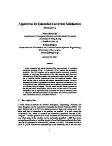
Figure 1. Semidefinite relaxation of Max Co-BIJ(d) with variable set X. A clause in the Max CoBIJ(d) instance is denoted by (x, x0 , π) where x ∈ X and x0 ∈ X are variables and π: Zd → Zd is a permutation. The clause is satisfied unless x = j and x0 = π(j) for some j ∈ Zd . Each clause (x, x0 , π) has a non-negative weight wx,x0 ,π associated with it.

Conclusions: We are not able to completely resolve the status of the 2-CSP problem over larger domains. Using reductions, we prove a hardness result of 1 − Ω(1/d2 ) for Max E2-Sat(d), which compares reasonably well with the (1−1/d2 ) random assignment threshold. For satisfiable instances of Max E2-Sat(d), we prove a hardness result of 1 − Ω(1/d3 ). Nevertheless, we conjecture that there is an approximation algorithm beating the random assignment threshold for Max E2-Sat(d), and hence for all instances of 2-CSP. Organization: We begin with a brief Section 2 highlighting why Max E2-Sat(d) is the hardest Max E2-CSP(d) problem in terms of beating the random assignment threshold. Next, in Section 3 we prove that every Max Co-BIJ(d) problem admits an algorithm that beats the random assignment threshold, and record some of its consequences. In Section 7, we prove that Max E3-NAE-Sat(G) is approximation resistant for most groups, including G = Zd (the case of most interest in the context of Max E2-Sat(d)). Finally, we record results that directly apply to Max E2-Sat(d) in Section 8.

2

The “Universality” of Max E2-Sat(d)

We note that the existence of an approximation algorithm that beats the random threshold for every 2-CSP is equivalent to the existence of such an algorithm for Max E2-Sat(d). Thus, an algorithm for Max E2-Sat(d) with performance ratio better than (1 − 1/d2 ) will imply that no 2-CSP is approximation resistant, thus resolving our conjecture that every 2-CSP is “easy”. This claim is seen by a “gadget” reducing an arbitrary CSP(d) to Max E2-Sat(d). Given an instance of any 2-CSP, construct an instance of Max E2-Sat(d) by repeating the following for every constraint C in the original 2-CSP: For every non-satisfying assignment to C, add one 2SAT(d) constraint which has precisely this non-satisfying assignment. If an assignment satisfies C then it also satisfies all the 2SAT(d) constraints in the gadget, and otherwise it satisfies precisely all but one of the 2SAT(d) constraints. Using this fact, it is straightforward to show that if Max E2-Sat(d) can be approximated beyond the random threshold, the above procedure gives an approximation algorithm that approximates an arbitrary 2-CSP beyond the random threshold. Conversely, if any 2-CSP at all is approximation resistant, then Max E2-Sat(d) must be approximation resistant.

4

1. 2. 3. 4. 5. 6.

Solve the semidefinite program in Fig. 1. Denote by uxj the vectors obtained from the solution. P x For every (x, j) ∈ X × Zd , let vjx = uxj − d1 d−1 j=0 uj . Select r from a dn-dimensional N(0, I) Gaussian distribution. Set qxj = d1 + Khr, vjx i for all (x, j) ∈ X × Zd . For each x ∈ X, – set pxj = qxj if qxj ∈ [0, 2/d] for all j ∈ Zd ; – set pxj = 1/d for all j ∈ Zd otherwise. 7. For each x ∈ X, let x = j with probability pxj . Figure 2. Approximation algorithm for Max Co-BIJ(d) with variable set X. The algorithm is parameterized by the positive constant K.

3

Approximation algorithm for Max Co-BIJ(d)

To construct an approximation algorithm for Max Co-BIJ(d) we combine a modification of the semidefinite relaxation used by Khot [12] for the Max BIJ(d) problem with a modification of the randomized rounding used by Andersson [1, 2] for the Max d-Section problem. Recall that a specific clause in the Max Co-BIJ(d) problem is of the form (x, x0 , π), where x and x0 are variables in the Max Co-BIJ(d) instance and π is a permutation, and that the clause is satisfied unless x = j and x0 = π(j) for some j. In our semidefinite relaxation of Max Co-BIJ(d) there are d vectors {ux0 , . . . , uxd−1 } for every variable x in the Max Co-BIJ(d) instance. Intuitively, the vector uxj sets the value of the variable x to j. To prove that our algorithm beats the random assignment threshold, we first establish that the semidefinite program in Fig. 1 is a relaxation of Max Co-BIJ(d), then prove that the rounding scheme proposed in Fig. 2 is well-defined, and finally analyze the expected performance of the rounding scheme using local analysis. Lemma 1. The semidefinite program in Fig. 1 is a relaxation of Max Co-BIJ(d). Proof. Suppose that we have an instance of Max Co-BIJ(d) with variable set X. Given an assignment ρ to the variables in X consider the following configuration of vectors: Let a be a vector of unit norm and define (

uxj =

a if j = ρ(x), 0 otherwise.

This configuration of vectors is feasible for the semidefinite program in Fig. 1 and the corresponding value of the objective function is exactly the weight of the satisfied equations in the Max Co-BIJ(d) instance. Lemma 2. Suppose that {uxj : (x, j) ∈ X × Zd } is a feasible solution to the semidefinite program in Fig. 1. Then the barycenter bx =

X 1 d−1 ux d j=0 j

of the vectors {uxj : j ∈ Zd }d−1 j=0 is independent of x. Proof. The constraints in the semidefinite program imply that |bx |2 = |bx0 |2 = hbx , bx0 i = d−2 .

5

Lemma 3. For any clause (x, x0 , π) in the Max Co-BIJ(d) instance, the algorithm in Fig. 2 satisfies (x, x0 , π) with probability at least 

1−

d−1 X

Z 

0

huxj , uxπ(j) i

B

j=0

1 K 2 r12 + dP (r) d d 

1−

0

where K is any positive constant, the vectors uxj and uxj 0 are as described in the algorithm, B = {r ∈ R2d : |r| ≤ 1/Kd}, and P is the probability distribution of a 2d-dimensional Gaussian with mean zero and identity covariance matrix. Proof. Consider an arbitrary clause (i, i0 , π) and the corresponding values qxj computed by the algorithm. Let B = {r ∈ R2d : |r| ≤ 1/Kd}. When r ∈ B, both qxj and qx0 j are in the interval [0, 2/d]; hence the clause (i, i0 , π) is satisfied with probability 1−

d−1 X

pxj px0 ,π(j) = 1 −

j=0

d−1 X

1 + Khr, vjx i d



j=0

1 x0 + Khr, vπ(j) i d



d−1 X 1 2 x0 =1− −K hr, vjx ihr, vπ(j) i d j=0 0

0

x i = hr, ux −bihr, ux given r in this case. By the definition of vjx from the algorithm, hr, vjx ihr, vπ(j) j π(j) − 0

0

bi = hr, uxj ihr, uxπ(j) i−hr, uxj ihr, bi−hr, uxπ(j) ihr, bi+hr, bihr, bi where b is the barycenter of the vectors {uxj : j ∈ Zd }, which is independent of x according to Lemma 2. Therefore −K 2

d−1 X



0

x hr, vjx ihr, vπ(j) i = K 2 dhr, bihr, bi −

j=0

d−1 X

0



hr, uxj ihr, uxπ(j) i .

j=0

To conclude, the probability that the clause is satisfied given r is d−1 X 1 0 + K 2 dhr, bihr, bi − hr, uxj ihr, uxπ(j) i d j=0



1−



(1)

when r ∈ B. Integrating over B, we can thus bound the probability that the clause is satisfied from below by Z B

d−1 X 1 0 1 − + K 2 dhr, bihr, bi − hr, uxj ihr, uxπ(j) i d j=0

!



dP (r).

To compute the integral of hr, bihr, bi, introduce an orthonormal basis {ek } such that b = e1 /d and P write r = k rk ek in this basis. Then 1 r2 dP (r) d2 B 1 B where the last integral is actually independent of the basis since both P and B are spherically sym0 metric. To compute the integral of hr, uxj ihr, uxπ(j) i, we proceed similarly: Introduce an orthonormal Z

hr, bihr, bi dP (r) =

Z

0

basis {ek } such that uxj = x1 e1 and uxπ(j) = y1 e1 + y2 e2 . Then Z B

0

hr, uxj ihr, uxπ(j) i dP (r) =

Z B

(r12 x1 y1 + r1 r2 x1 y2 ) dP (r).

6

The integral of the second term vanishes since the integrand is odd and the interval is symmetric around the origin. Therefore Z

0

B

hr, uxj ihr, uxπ(j) i dP (r) = x1 y1

Z B

0

r12 dP (r) = huxj , uxπ(j) i

Z B

r12 dP (r).

To conclude, we can write the probability that the clause is satisfied as a − cx where Z 

a= B

c = K2

Z B

x=

d−1 X

1 K 2 r12 + dP (r), d d 

1−

r12 dP (r), 0

huxj , uxπ(j) i.

j=0

We now find an α such that a − cx ≥ α(1 − x). Since the expression (1) is a probability it is non-negative for every r. Hence a ≥ c ≥ 0 and, since the constraints in the semidefinite program imply that x ≥ 0, 

a − cx ≥ a − ax = 1 −

d−1 X

0

Z 

huxj , uxπ(j) i

B

j=0

1 K 2 r12 + dP (r). d d 

1−

√ Theorem 1. The algorithm in Fig. 2 with K = 1/ 13d3 is a randomized polynomial time approximation algorithm for Max Co-BIJ(d) with expected performance ratio 1 − d−1 + 0.07d−4 and thus better than the random assignment threshold. Proof. Consider the algorithm in Fig. 2 applied to an instance of Max Co-BIJ(d). By Lemma 1, the semidefinite program in Fig. 1 is a relaxation of Max Co-BIJ(d); therefore the optimum value of the Max Co-BIJ(d) instance can be bounded by 

X

wx,x0 ,π 1 −

x,x0 ,π

d−1 X

0



huxj , uxπ(j) i

j=0

where the vectors uxj are the solution to the program. Now consider the rounding. By Lemma 3, the clause (x, x0 , π) is satisfied with probability 

1−

d−1 X

0

Z 

huxj , uxπ(j) i

j=0

B

1 K 2 r12 + dP (r) d d 

1−

By Lemmas 21 and 22, Z  B

1 K 2 r12 1 0.07 1− + dP (r) ≥ 1 − + 4 d d d d 

with the parameter choice K 2 = d−3 /13. So with this parameter choice, it now follows by linearity of expectation and the above bound on the optimum value of the Max Co-BIJ(d) instance that the expected weight of the solution produced by the algorithm is at least a factor (1 − d−1 + 0.07d−4 ) times the optimum value of the Max Co-BIJ(d) instance.

7

1. Select a random assignment ρ to the variables in the instance. 2. Replace each equation ax + by = c with the d − 1 inequations ax + by 6= ci for all ci 6= c. Obtain an assignment τ by running the algorithm in Fig. 2 on this instance. 3. Pick the best of the assignments ρ and τ . Figure 3. Approximation algorithm for Max E2-Lin(d).

3.1

An approximation algorithm for Max E2-Lin(d)

We can use the above algorithm for Max Co-BIJ(d) to construct an algorithm also for Max E2Lin(d): Simply replace an equation ax + by = c with the d − 1 inequations ax + by 6= ci for all ci 6= c. Then an assignment that satisfies a linear equation satisfies all of the corresponding linear inequations and an assignment that does not satisfy a linear equation satisfies d − 2 of the d − 1 corresponding linear equations. This algorithm gives a performance ratio of 1/d + Ω(1/d4 ) which improves significantly on the previously best known ratio of 1/d + Ω(1/d14 ) [3]. Theorem 2. For all d ≥ 4, the algorithm in Fig. 3 is a randomized polynomial time approximation algorithm for Max E2-Lin(d) with expected performance ratio d−1 + 0.05d−4 . Proof. If the optimum of the instance is smaller than a fraction 1 − 0.05d−3 of all equations, the random assignment—which satisfies an expected fraction 1/d of all equations—satisfies an expected fraction 1/d 1 0.05 ≥ + 4 −3 1 − 0.05d d d of the optimum. If the optimum is larger than a fraction 1 − 0.05d−3 of all equations, the optimum of the instance of inequations is at least 1−0.05d−3 (d−1)−1 . By Theorem 1, our approximation for Max Co-BIJ(d) from Fig. 2 therefore finds a solution with expected weight at least a fraction 

0.05 1− 3 d (d − 1)



d − 1 0.07 + 4 d d



=

d − 1 0.02 0.0035 + 4 − 7 d d d (d − 1)

of all inequations. An assignment satisfying a fraction 1/d + α of the equations satisfies a fraction d−2 1 d−1 α 1 +α + 1− −α = + d d−1 d d d−1 of the inequations and vice versa; therefore the assignment constructed above satisfies at least an expected fraction 







1 0.02(d − 1) 0.0035 1 0.02(d − 1 − 0.0035d−3 ) + − > + d d4 d7 d d4 of the equations. The function d−1−0.0035d−3 is increasing in d and for d = 4 it is 3−0.0035/64 > 2.5. Therefore, at least an expected fraction d−1 + 0.05d−4 of all equations are satisfied when d ≥ 4. Corollary 1. For all d ≥ 2, there is a polynomial time approximation algorithm for Max E2-Lin(d) with expected performance ratio d−1 +0.05d−4 and thus better than the random assignment threshold.

8

Repeat the following for every relation in the Max Co-BIJ(d) instance: 1. 2. 3. 4. 5. 6.

Let R be the bipartite graph defined by the relation. Let r be the degree of R. Let Rc be the complement of R. Decompose the edges of Rc into perfect matchings R1 , . . . , Rd−r . Define the relations πi such that d1 ∼πi d2 if (d1 , d2 ) ∈ Ri . Add the relations π1 , π2 , . . . , πd−r to the Max Co-BIJ(d) instance.

Figure 4. Construction of an instance of Max Co-BIJ(d) from an instance of any regular CSP.

1. Select a random assignment ρ to the variables in the instance. 2. Create an instance of Max Co-BIJ(d) as described in Fig. 4. Obtain an assignment τ by running the algorithm in Fig. 2 on this instance. 3. Pick the best of the assignments ρ and τ . Figure 5. Approximation algorithm for any regular CSP.

Proof. Algorithms for d = 2 and d = 3 have been provided by Goemans and Williamson [8, 9], for d ≥ 4 the result follows by Theorem 2

3.2

An approximation algorithm for regular 2-CSPs

We can obtain an approximation algorithm for all regular CSPs by a straightforward generalization of the ideas from the previous section. Given an r-regular 2-CSP, we proceed as follows for every relation R defining the CSP: Decompose Rc , the “bipartite complement” of the graph defined by R, 1 , π 2 , . . . , π d−r . Then let these matchings define the Max Co-BIJ(d) into (d − r) perfect matchings πR R R instance. An assignment that satisfies R satisfies all of the d − r matchings while an assignment that does not satisfy R satisfies d − r − 1 of them. Run the following two algorithms and take the assignment producing the largest weight as the result: The first algorithms selects a random assignment to the variables; the second algorithm runs the above algorithm for Max Co-BIJ(d). Theorem 3. For all d ≥ 2 and all 1 ≤ r ≤ d−1, the algorithm in Fig. 5 is a randomized polynomial time approximation algorithm for r-regular CSPs with expected performance ratio r/d + Ω(d−4 ). Proof. Consider the result of the algorithm on an arbitrary instance. If the optimum of the instance is smaller than a fraction 1−0.05(d−r)d−3 (d−1)−1 of all equations, the random assignment—which satisfies an expected fraction r/d of all equations—satisfies an expected fraction r 0.05r(d − r) r/d ≥ + 4 1 − 0.05(d − r)d−3 (d − 1)−1 d d (d − 1) of the optimum.

9

If the optimum is larger than a fraction 1 − 0.05(d − r)d−3 (d − 1)−1 of all constraints, the optimum of the corresponding instance of Max Co-BIJ(d) is at least a fraction d−r−1 0.05(d − r) 1− 1− 3 d (d − 1) d−r 



=1−

0.05 − 1)

d3 (d

By Theorem 1, our approximation for Max Co-BIJ(d) from Fig. 2 therefore finds a solution with expected weight at least a fraction 

0.05 1− 3 d (d − 1)



d − 1 0.07 + 4 d d



=

d − 1 0.02 0.0035 + 4 − 7 d d d (d − 1)

of all constraints in the Max Co-BIJ(d) instance. An assignment satisfying a fraction r/d + α of the constraints in the r-regular CSP satisfies a fraction d−r−1 r d−1 α d−r r +α + 1− −α = + d−r d d−r d d d−r 







of the constraints in the Max Co-BIJ(d) instance and vice versa; therefore the assignment constructed above satisfies at least a fraction r 0.02(d − r) 0.0035(d − r) + − d d4 d7 (d − 1) of the constraints in the r-regular CSP. It is not necessary that the various constraints be r-regular for the same r, and a similar argument also shows that every regular 2-CSP can be approximated in polynomial time beyond its random assignment threshold.

4

PCPs and inapproximability results: Background

In his seminal paper [10], Håstad introduced a methodology for proving inapproximability results for constraint satisfaction problems. On a high level, the method can be viewed as a simulation of the well-known two-prover one-round (2P1R) protocol for E3-Sat where the verifier sends a variable to one prover and a clause containing that variable to the other prover, accepting if the returned assignments are consistent and satisfy the clause.

4.1

The 2-prover 1-round protocol

We start with an instance of the NP-hard [4, 6] problem µ-gap E3-Sat(5). Definition 3. µ-gap E3-Sat(5) is the following decision problem: We are given a Boolean formula φ in conjunctive normal form, where each clause contains exactly three literals and each literal occurs exactly five times. We know that either φ is satisfiable or at most a fraction µ < 1 of the clauses in φ are satisfiable and are supposed to decide if the formula is satisfiable. There is a well-known two-prover one-round (2P1R) interactive proof system that can be applied to µ-gap E3-Sat(5). It consists of two provers, P1 and P2 , and one verifier. Given an instance, i.e., an E3-Sat formula φ, the verifier picks a clause C and variable x in C uniformly at random from the instance and sends C to P1 and x to P2 . It then receives an assignment to the variables in C from P1 and an assignment to x from P2 , and accepts if these assignments are consistent and satisfy C. If the provers are honest, the verifier always accepts with probability 1 when φ is satisfiable, i.e., the proof system has completeness 1, or perfect completeness. It can be shown that the provers can fool 10

the verifier with probability at most (2 + µ)/3 when φ is not satisfiable, i.e., that the above proof system has soundness (2 + µ)/3. The soundness can be lowered to ((2 + µ)/3)u by repeating the protocol u times independently, but it is also possible to construct a one-round proof system with lower the soundness by repeating u times in parallel as follows: The verifier picks u clauses (C1 , . . . , Cu ) uniformly at random from the instance. For each Ci , it also picks a variable xi from Ci uniformly at random. The verifier then sends (C1 , . . . , Cu ) to P1 and (x1 , . . . , xu ) to P2 . It receives an assignment to the variables in (C1 , . . . , Cu ) from P1 and an assignment to (x1 , . . . , xu ) from P2 , and accepts if these assignments are consistent and satisfy C1 ∧ · · · ∧ Cu . As above, the completeness of this proof system is 1, and it can be shown [15] that the soundness is at most cuµ , where cµ < 1 is some constant depending on µ but not on u or the size of the instance.

4.2

Constructing strategies for the provers

In the above setting, the proof is simply an assignment to all the variables. In that case, the verifier can just compare the assignments it receives from the provers and check if they are consistent and satisfying. The construction we use to prove that several non-Boolean constraint satisfaction programs are non-approximable beyond the random assignment threshold can be viewed as a simulation of the u-parallel repetition of the above 2P1R interactive proof system for µ-gap E3-Sat(5). We use a probabilistically checkable proof system (PCP) with a verifier closely related to the particular constraint we want to analyze. To find predicates that depend on variables from some domain of size d and are non-approximable beyond the random assignment threshold, we work with an Abelian group of order d. That enables us to use representation theory for Abelian groups to analyze our protocols. The final verifier expects as proof encodings of the answers of P1 and P2 in the Raz 2P1R, and then checks very efficiently, by making very few queries, that the proof is close to valid encodings of answers that would have made the 2P1R verifier accept with good probability. To get hardness results for CSPs over domain size d, the specific encoding used is the so called long G-code, which will be defined in Sec. 6, for some Abelian group G of order d. The proof expected by the PCP verifier consists of purported Long G-Codes of the assignments to the variables in U and W for each possible choice (U, W ) of the 2P1R verifier. The PCP design task thus reduces to designing an “inner” verifier to check if two purported Long G-Codes encode assignments which are consistent answers for P1 and P2 in the 2P1R. One designs such a verifier with an acceptance predicate closely tied to the problem at hand, and its performance is analyzed using Fourier analysis. The basic strategy here is to show how proofs that make the “inner” verifier accept with high probability can be used to extract good strategies for P1 and P2 in the 2P1R protocol. On a high level, the Fourier expansion of the purported long codes are used to extract probabilistic strategies for the provers P1 and P2 . We are able to express the acceptance probability of the verifier in the 2P1R protocol as a sum of certain pairwise products of Fourier coefficients and these products turn out to be large whenever the “inner” verifier accepts with large probability. On a slightly more detailed level, let w be the probability that the considered constraint is satisfied by a random assignment. The aim of our analysis is to prove that it is NP-hard to satisfy more than a fraction w of the constraints. We do this by proving the contrapositive: If we can satisfy a fraction w + ε of the constraints, for any constant ε > 0, we can decide any language in NP in polynomial time. This follows from the connection between our PCP and the 2P1R interactive proof system for µ-gap E3-Sat(5): We assume that it is possible to satisfy a fraction w + ε for some constant ε > 0 and prove that this implies that there is a correlation between the

11

tables queried by the verifier in our PCP. We can then use this correlation to explicitly construct strategies for the provers in the 2P1R proof system for µ-gap E3-Sat(5) such that the verifier in that proof system accepts with probability that is independent of u. By selecting u large enough, we can then reach a contradiction. The final link in the chain is the observation that since our verifier uses only logarithmic randomness, we can form a CSP with polynomial size by enumerating the checked constraints for every possible outcome of the random bits. If the resulting constraint satisfaction program is approximable beyond the random assignment threshold, we can use it to decide the NP-hard language µ-gap E3-Sat(5) in polynomial time.

5

Representation theory and the Fourier transform

In this section we give a brief account of the representation theory for Abelian groups and the associated Fourier transform. For more details, we refer the reader to Terras’s book [16]. In this paper, we always denote groups by the letters F , G and H, members in those groups by lowercase ˆ and H ˆ by lowercase Greek Roman letters and members in the corresponding dual groups Fˆ , G letters.

5.1

Representation theory for Abelian groups

ˆ be its dual group, i.e., the group of all homomorphisms from G Let G be an Abelian group and G ˆ on a member to C. A central concept in the representation theory is the action of a member of G of G. Since the dual groups consists of functions from G to C, such an action is simply the evaluation ˆ at a member of G. of a member of G Example 1. The group Zd for some positive integer d is isomorphic to the group consisting of powers of e2πi/d with multiplication as the group operation and 1 as identity. The dual group then consists of all functions x 7→ xn for the integers n from 0 to d − 1. The product of the functions x 7→ xn and x 7→ xm is the function x 7→ xm+n , where addition is defined modulo d. This implies that the trivial homomorphism, that maps every group element to 1 and thus is the function x 7→ x0 , is the identity in the dual group. ˆ we The above example motivates the following notation in the general case: For g ∈ G and γ ∈ G γ let g denote γ(g). We let multiplication be the group operation in G and addition be the group ˆ and denote the identities by 1 and 0, respectively. Then we can write the following operation in G γ 1 identities: g g γ2 = g γ1 +γ2 , g1γ g2γ = (g1 g2 )γ , (g 2 )γ = g 2γ = g γ g γ , g −γ = (g −1 )γ , g 0 = 1, 1γ = 1. We also need the following symmetry relations: ( X

γ

g =

g∈G

5.2

|G| if γ = 0, 0 otherwise,

( X

γ

g =

ˆ γ∈G

|G| if g = 1, 0 otherwise.

The Fourier transform

Now let f be a function from G to C. Then we can write f as a Fourier series f (g) =

X

fˆγ g γ

(2)

ˆ γ∈G

where 1 X fˆγ = f (g)g −γ . |G| g∈G

(3)

12

Moreover the following version of Plancherel’s equality holds in this case: X

|fˆγ |2 =

ˆ γ∈G

6

1 X |f (g)|2 . |G| g∈G

(4)

The long G-code and its Fourier transform

Recall that our construction should simulate the 2P1R game for 3-Sat where the verifier sends u clauses to one prover and one variable from each clause to the other prover. Our proof, encoded by the long G-code, should contain these queries for all possible choices of the verifier in the 2P1R game. Since the verifier in the 2P1R games always rejects if it receives an answer which does not satisfy the u clauses we can in fact assume that the clause-prover always returns a satisfying assignment. Our encoding of the proof also reflects this in a way that will now be made explicit. Definition 4. Let U be a set of variables and denote by {−1, 1}U the set of assignments to the variables in U . The long G-code of some x ∈ {−1, 1}U is a function AU,x : {−1, 1}U → G defined by AU,x (f ) = f (x). Definition 5. Let W be a set of clauses and denote by SATW the set of satisfying assignments to the clauses in W . The long G-code of some y ∈ SATW is a function AW,y : SATW → G defined by AW,y (h) = h(y). Definition 6. A standard written G-proof with parameter u contains for each sequence U of u variu U ables a string of length |G|2 , which we interpret as the table of a function AU : G{−1,1} → G. It u also contains for each set W of u clauses a string of length |G|7 which we interpret as the table of W a function AW : GSAT → G. Definition 7. A standard written G-proof with parameter u is a correct proof for a formula φ if there is an assignment x, satisfying φ, such that AV is the long G-code of x|V for any sequence V of u variables or any sequence V of u clauses. The verifier in our PCPs will typically select a random sequence W of clauses and then form U by selecting a variable at random from each clause. It will then query the tables AU and AW in the standard written G-proof at cleverly chosen positions. We analyze the verifier using the Fourier expansion of the alleged long codes; we therefore need to understand the Fourier transform of functions from GI to C for some finite set I. Since the Fourier coefficients are used to devise a strategy for the provers in the 2P1R game, certain Fourier coefficients must be identically zero. The analysis also needs certain facts regarding the Fourier transform of two functions A: GI → C and B: GJ → C where there is a projection from J to I. All these identities have already been obtained by Håstad [10, § 2.6], we only state them here for easy reference. Let I be a finite set and consider the space GI , i.e., the space of all functions from I to G. This space can be identified with the group F = G|I| since a function is simply a table of all its values for all of the |I| possible inputs. Then the products of two functions is just the products of the corresponding group elements, and so on. For an element f ∈ F and an element x ∈ I, we let f (x) denote the coordinate in f corresponding to x. Now let A be a function from F to C. We can write this function as a Fourier series A(f ) =

X

Aˆα f α .

α∈Fˆ

13

ˆ then we can To describe the elements of Fˆ , it is convenient to view them as functions from I to G; write fα =

Y

(f (x))α(x) .

x∈I

ˆ The latter expression is well-defined since f (x) ∈ G and α(x) ∈ G. ˆ if A(gf ) = g γ A(f ) for all g ∈ G. Definition 8. A function A: F → C is γ-homogeneous for γ ∈ G Lemma 4. Let F = GI and suppose that A: F → C is γ-homogeneous. Let Aˆα be the Fourier P coefficients of A. Then Aˆα = 0 unless γ = i∈I α(i). In particular, Aˆ0 = 0 if γ = 6 0. Now let J be a finite set satisfying |I| ≤ |J| and π: J → I be an onto mapping. Consider the space H = GJ . Any f ∈ F , i.e., any function from I to G can then be transformed in a canonical way to a function from J to G, i.e., to a member of H, by composing it with π; we denote this new ˆ i.e., a function from H to C can be associated in a natural function by f ◦ π. Similarly, a β ∈ H, way with a function from F to H, i.e., with a member of Fˆ . We denote this new function by πG (β) and it is defined in such a way that πG (β), viewed as a homomorphism from F to C, is the map P f 7→ (f ◦ π)β . It is easy to see that if α = πG (β) then it holds that α(i) = j∈π−1 (i) β(j) for all i ∈ I. Lemma 5. Given an Abelian group G, two finite sets I and J such that |I| ≤ |J| and an onto ˆ (f ◦ π)β = f πG (β) . mapping π: J → I, let F = GI and H = GJ . Then, for any β ∈ H, As we already mentioned, in our case I = {−1, 1}U and J = SATW for some sequence W of u variables and some sequence U formed by selecting a variable from each clause in W . Our analysis involves the Fourier transform of functions γ ◦ AU and γ ◦ AW and it turns out that we need those functions to be γ-homogeneous. This can be enforced by certain access conventions in the verifier. Definition 9. A function A from F to G is folded over G if A(gf ) = gA(f ) for all g ∈ G. Lemma 6. If A is folded over G, then γ ◦ A is γ homogeneous. We can assume that all tables in the proof are folded since this can be simulated with the following access convention in the verifier: Partition GF into equivalence classes by the relation ≡, where f ≡ h if there is g ∈ G such that f = gh, i.e., ∀w(f (w) = gh(w)). Write [f ] for the equivalence class of f . Then, whenever the position corresponding to some function h is queried, return gA(f ) where g and f are such that h = gf and f is the chosen representative for [h].

7

Inapproximability results for Max E3-NAE-Sat(G)

In this section, our aim is to prove that unlike the Boolean case, for every d ≥ 3, Max E3-NAESat(Zd ) is approximation resistant. We will actually prove that Max E3-NAE-Sat(G) is approximation resistant for pretty much every finite Abelian group. Theorem 4 (Main hardness result). For every constant ε > 0 and every finite Abelian group G that is not isomorphic to Z2m for any positive integer m, it is NP-hard to distinguish instances of Max E3-NAE-Sat(G) that are satisfiable from instances where at most a fraction (1 − |G|−2 + ε) of the constraints are simultaneously satisfiable. 14

As a warm-up, we first prove the easier result that Max E3-LinInEq(G) is approximation resistant, even with perfect completeness, for every finite Abelian group of order at least three. This result can be used together with a simple gadget to prove that Max E3-NAE-Sat(Z3 ) is approximation resistant. To prove the same result for all finite Abelian groups, we proceed in three stages: We first treat all groups of odd order, then Z2m for m ≥ 2, and finally treat all groups by combining the proofs for the first two cases. In all our protocols we use the following notation: Convention 1. When analyzing a PCP that tests if some µ-gap E3-Sat(5) formula Φ is satisfiable, expectations over U and W range over all sequences W of u clauses from Φ, with uniform measure, and all sequences U formed by selecting, uniformly and independently, one variable from each clause W U in W . Given U and W , we define the shorthands F = G{−1,1} , H = GSAT and let π be the projection that constructs an assignment in {−1, 1}U from an assignment in SATW .

7.1

Intuition behind our PCP constructions

A verifier in a PCP typically first selects sets U and W uniformly at random and then checks a small number of positions in tables corresponding to U and W . Specifically, the standard way to get a PCP with three queries is to query one position in a table corresponding to U and two positions in a table corresponding to W . The three values obtained are then tested to see if they satisfy some given constraint—such a construction gives a hardness result for the CSP corresponding to the type of constraint checked. To get a hardness result for Max E3-NAE-Sat(G) the constraint checked by the verifier therefore has to be a not-all-equal constraint. Moreover, we want the verifier to have perfect completeness, i.e., to always verify a correct proof. We accomplish this by querying the positions AU (f ), AW (h) and AW (f −1 h2 e) where f and h are selected uniformly at random and e is selected such that e(y) is selected independently and uniformly at random from G \ {1}. Here, the function f −1 h2 e is the map y 7→ (f (y|U ))−1 (h(y))2 e(y). For a correct proof of a satisfying assignment, the answers to these queries will be f (y|U ), h(y) and (f (y|U ))−1 (h(y))2 e(y) where y is a satisfying assignment to the clauses in W . These three values can never be all equal, since f (y|U ) = h(y) implies that (f (y|U ))−1 (h(y))2 e(y) = h(y)e(y) 6= h(y). Therefore the verifier always accepts a correct proof and to prove that it accepts a proof corresponding to an unsatisfying assignment with probability at most 1 − |G|−2 + ε, where ε > 0 is an arbitrary constant, we proceed as follows: The assumption that the verifier accepts with probability 1 − |G|−2 + ε implies that a sum of certain pairs of related Fourier coefficients is large. Those coefficients can be used to devise strategies for the provers in the u-parallel version of the 2P1R game for µ-gap E3-Sat(5), strategies that make the verifier of that game accept with probability independent of u. This leads to a contradiction since it is known [15] that this protocol as soundness cuµ . The precise coupling can be expressed as follows: ˆ \ {0} is arbitrary and that AU Lemma 7. Given a finite Abelian group G, suppose that γ ∈ G and AW are the folded tables of a standard written G-proof with parameter u that corresponds to an unsatisfiable instance of µ-gap E3-Sat(5). Then EU,W

X



ˆβ |2 |β|−1 < η, |AˆπG (β) |2 |B

ˆ β∈H

where U , W , F , H, and π are as in Convention 1, A = γ ◦ AU , and B = γ ◦ AW , provided that u > log η/ log cµ .

15

The proof is a standard written G-proof with parameter u: The verifier acts as follows: 1. Select a sequence W of clauses, each clause uniformly and independently at random from Φ. 2. Select a sequence U of variables by selecting one variable from each clause in W , uniformly and independently. 3. Let π: SATW → {−1, 1}U be the function that creates an assignment in {−1, 1}U from an assignment in SATW . W U 4. Let F = G{−1,1} and H = GSAT . 5. Select f ∈ F and h ∈ H uniformly at random. 6. Select e ∈ H such that independently for every y ∈ SATW , e(y) is uniformly distributed in G \ {1}. 7. Accept if AU (f )AW (h)AW ((f ◦ π)−1 h−1 e) 6= 1; Reject otherwise. Figure 6. The PCP used to prove optimal approximation hardness for Max E3-LinInEq(G) for any finite Abelian group G such that |G| ≥ 3. The PCP is parameterized by the constant u and tests if a µ-gap E3-Sat(5) formula Φ is satisfiable.

Proof. We use the tables to construct strategies for the provers in the 2P1R game as follows: The ˆ \ {0} that maximizes provers first compute the γ ∈ G EU,W

X

ˆβ |2 |β|−1 |AˆπG (β) |2 |B



ˆ β∈H

and keep this γ fixed. Given a sequence U of variables, the second prover computes the Fourier coefficients Aˆα selects an α according to probability distribution given by |Aˆα |2 and then an x such that α(x) 6= 0 uniformly; this x is returned to the verifier. ˆβ selects a β Given a sequence W of clauses, the first prover computes the Fourier coefficients B ˆβ |2 and then a y such that β(y) 6= 0 uniformly; according to probability distribution given by |B this y is returned to the verifier. The assignment y always satisfies the clauses in W and it is guaranteed to be consistent if α = πG (β) and the second prover happens to select precisely the y that projects onto the x selected by the first prover. Therefore, the success probability of the above strategy is at least EU,W

X



ˆβ |2 |β|−1 . |AˆπG (β) |2 |B

ˆ β∈H

Since it is known that the soundness of the 2P1R game is at most cuµ and the above expression is independent of u, the conclusion follows by selecting u > log η/ log cµ .

7.2

Warm-up: Linear inequations

The PCP is described in Fig. 6. The setting is as usual; the verifier first picks u clauses of the 3SAT instance at random and then a variable from each clause at random. It then queries three positions in tables in the proof that should correspond to an assignment to the clauses and variables and accepts if a certain inequation is satisfied. Perfect completeness follows easily: 16

Lemma 8. The verifier in Fig. 6 has perfect completeness. Proof. Suppose that the proof is the correct encoding of some satisfying assignment y. Then AU (f ) = f (y|U ) and AW (h) = h(y|W ), hence AU (f )AW (h)AW ((f ◦ π)−1 h−1 e) = e(y|W ) 6= 1 and the verifier accepts. Let us now study the error function e selected by the verifier. Lemma 9. Let e be picked as in Fig. 6 applied to a finite Abelian group of order at least three. Then | E[eβ ]| ≤ 2−|β| , where |β| is defined as the size of the support of β, i.e., the number of y such that β(y) 6= 0. Proof. Since e is selected in such a way that the e(y) are independent, i Y h β(y) E (e(y)) .

| E[eβ ]| =

y∈H

g0

Since factors

= 1 for all g ∈ G, the only factors that contribute are those where β(y) 6= 0. For those

h

i

E (e(y))β(y) =

X 1 −1 g β(y) = , |G| − 1 g∈G\{1} |G| − 1

where the last equality follows since

P

g∈G g

γ

= 0 for all γ 6= 0. Hence

| E[eβ2 ]| = (|G| − 1)−|β| ≤ 2−|β| . The soundness is straightforward to analyze using the now standard methodology introduced by Håstad [10]. As usual, we assume that the test accepts with probability 1 − |G|−1 + δ and prove that the tables in the proof must then be correlated. We then use this correlation to extract strategies for the provers in the 2P1R game. Lemma 10. Suppose that the verifier in Fig. 6 accepts with probability 1−|G|−1 +δ for some δ > 0. ˆ \ {0} such that Then there exists some γ ∈ G EU,W

X



ˆβ |2 4−|β| ≥ δ 2 , |AˆπG (β) |2 |B

ˆ β∈H

where U , W , F , H, and π are as in Convention 1, Aˆα are the Fourier coefficients of γ ◦ AU , and ˆβ are the Fourier coefficients of γ ◦ AW . B Proof. The suggested test accepts unless AU (f )AW (h)AW ((f ◦ π)−1 h−1 e) = 1, therefore we can write Pr[accept] = 1 −

X  1 E (AU (f )AW (h)AW ((f ◦ π)−1 h−1 e))γ |G| ˆ γ∈G

17

1 1 − E |G| |G|



=1−



(AU (f )AW (h)AW ((f ◦ π)−1 h−1 e))γ .

X

ˆ γ∈G\{0}

ˆ such that Now suppose that Pr[accept] ≥ 1 − |G|−1 + δ; then there exists a γ ∈ G   E (AU (f )AW (h)AW ((f ◦ π)−1 h−1 e))γ ≥ δ.

Now expand γ ◦ AU and γ ◦ AW in their Fourier series for this value of γ: (γ ◦ AU )(f ) =

X

Aˆα f α ,

(γ ◦ AW )(h) =

α∈Fˆ

X

ˆ β hβ . B

ˆ β∈H

This gives  X X X

δ ≤ E

h

ˆβ B ˆβ E f α hβ1 ((f ◦ π)−1 h−1 e)β2 Aˆα B 1 2

ˆ β2 ∈ H ˆ α∈Fˆ β1 ∈H

i

X X X h i α−πG (β2 ) β1 −β2 β2 ˆ ˆ ˆ = E Aα Bβ1 Bβ2 E f h e ˆ β2 ∈H ˆ α∈Fˆ β1 ∈H

X X X h i h i h i α−πG (β2 ) β1 −β2 ˆ ˆ ˆ = E Aα Bβ1 Bβ2 E f E h E eβ2 . ˆ β2 ∈H ˆ α∈Fˆ β1 ∈H

The first of the inner expectations is zero unless α = πG (β2 ), the second of the inner expectations is zero unless β1 − β2 = 0. Putting this together, we get the bound  2

 X

δ 2 ≤ E

ˆ β∈H

ˆ 2 E[eβ ] AˆπG (β) B β

" 2 # X ˆ 2 E[eβ ] AˆπG (β) B ≤ E β ˆ β∈H

"

≤E

X

ˆβ |2 | E[eβ ]|2 |AˆπG (β) |2 |B

 X

ˆ β∈H

X

=E

ˆβ |2 |B

#

ˆ β∈H

ˆβ |2 | E[eβ ]|2 |AˆπG (β) |2 |B



ˆ β∈H

X

≤E



ˆβ |2 4−|β| , |AˆπG (β) |2 |B

ˆ β∈H

where the equality follows since X X ˆβ |2 = 1 |(AW (h))γ |2 = 1 |B |H| h∈H ˆ β∈H

by Plancherel’s equality. Theorem 5. For every constant ε > 0 and every finite Abelian group G such that |G| ≥ 3, it is NP-hard to distinguish instances of Max E3-LinInEq(G) that are satisfiable from instances where at most a fraction (1 − |G|−1 + ε) of the inequations are simultaneously satisfiable.

18

The proof is a standard written Zd -proof with parameter u: The verifier acts as follows: Steps 1–6 are as in Fig. 6 applied to G = Zd . 7. Accept if AU (f ), AW (h) and AW ((f ◦ π)−1 h2 e) are not all equal; Reject otherwise. Figure 7. The PCP used to prove optimal approximation hardness for Max E3-NAE-Sat(Zd ) for odd d. The PCP is parameterized by the constant u and tests if a µ-gap E3-Sat(5) formula Φ is satisfiable.

Proof. Given ε, select u > 2 log ε/ log cµ . Then Lemmas 10 and 7 together imply that the soundness of the PCP in Fig. 6 has soundness at most 1 − |G|−1 + ε. Corollary 2. Max E3-NAE-Sat(Z3 ) is hard to approximate within 8/9+ε with perfect completeness for any ε > 0. Proof. We reduce Max E3-LinInEq(3), which we know to be hard to approximate within 2/3 with perfect completeness from Theorem 5 applied to the group Z3 , to Max E3-NAE-Sat(Z3 ). A clause x+y+z 6= 0 mod 3 is replaced with the clauses NAE(x, y, z), NAE(x+2, y+1, z), NAE(x+1, y+2, z). If all three NAE clauses are satisfied, then x + y + z 6= 0 mod 3; if x + y + z = 0 two of the NAE clauses are satisfied. Therefore it is hard to distinguish the case when all the constraints are satisfied from the case when a fraction 3(2/3 + 3ε) + 2(1/3 − 3ε) = 8/9 + ε 3 of the constraints are satisfied.

7.3

Case I: Groups of odd order

The PCP is described in Fig. 7. The setting is the same as in Sec. 7.2 but the acceptance predicate of the verifier is different. Lemma 11. The verifier in Fig. 7 has perfect completeness. Proof. Suppose that the proof is the correct encoding of a satisfying assignment. We get two cases: If AU (f ) = f (y|U ) and AW (h) = h(y|W ) are not equal, the verifier accepts; if f (y|U ) = h(y|W ), then AW ((f ◦ π)−1 h2 e) = h(y|W )e(y|W ) 6= h(y|W ) = AW (h) and the verifier accepts. The soundness is a bit more complicated to analyze. As usual, we assume that the test accepts with probability 1 − |G|−2 + δ and prove that the tables in the proof must then be correlated. We then use this correlation to extract strategies for the provers in the 2P1R game. Lemma 12. Suppose that the verifier in Fig. 7 accepts with probability 1−|G|−2 +δ for some δ > 0. ˆ \ {0} and γ2 ∈ G ˆ \ {0} such that Then there exists γ1 ∈ G EU,W

X



ˆβ |2 4−|β| ≥ δ 2 , |AˆπG (β) |2 |B

ˆ β∈H

where U , W , F , H, and π are as in Convention 1, Aˆα are the Fourier coefficients of γ1 ◦ AU , and ˆβ are the Fourier coefficients of γ2 ◦ AW . B

19

Proof. The test accepts unless all three queries return the same value, therefore we can write the P acceptance probability as 1 − g∈G E[Ig ] where Ig denotes the indicator for the event that all three queries return g: X 1 1 + (g −1 AU (f ))γ1 Ig = 3 |G| γ 6=0 



1+

X

1+

(g

−1

γ2

AW (h))



×

γ2 6=0

1



X 

(g −1 AW ((f ◦ π)−1 h2 e))γ3 .

γ3 6=0

We now expand the products and get X 1 1+ (g −1 AU (f ))γ1 3 |G| γ 6=0 

Ig =

1

+

X

(g

−1

AW (h))γ2 +

+

(g

−1

(g −1 AW ((f ◦ π)−1 h2 e))γ3

γ3 6=0 γ1 −1

γ2 6=0

X X

X

AU (f )) (g

AW (h))γ2

γ1 6=0 γ2 6=0

+

X X

(g −1 AU (f ))γ1 (g −1 AW ((f ◦ π)−1 h2 e))γ3

γ1 6=0 γ3 6=0

+

X X

(g −1 AW (h))γ2 (g −1 AW ((f ◦ π)−1 h2 e))γ3

γ2 6=0 γ3 6=0

+

X X X



(g −1 AU (f ))γ1 (g −1 AW (h))γ2 (g −1 AW ((f ◦ π)−1 h2 e))γ3 .

γ1 6=0 γ2 6=0 γ3 6=0

Let us now consider the contributions of the above terms when we sum Ig over all g ∈ G. The constant term contributes |G|/|G|3 = 1/|G|2 . The linear terms vanish since X

X

(gh)γ

g∈G γ∈G\{0} ˆ

where h is independent of g can be rewritten as X

hγ

X

gγ = 0

g∈G

ˆ γ∈G\{0}

where the equality follows since g∈G g γ = 0 for every γ 6= 0. The quadratic terms also disappear, but the argument is somewhat more involved. Consider terms of the first form: P

X X X

(g −1 AU (f ))γ1 (g −1 AW (h))γ2

g∈G γ1 6=0 γ2 6=0

=

X X

(AU (f ))γ1 (AW (h))γ2

γ1 6=0 γ2 6=0

X

g −γ1 −γ2 .

g∈G

For fixed, γ1 and γ2 such that γ1 + γ2 6= 0, the inner sum is definitely 0. Therefore, we only have to care about X ˆ γ∈G\{0}

h

i

E (AU (f ))γ (AW (h))−γ =

X

X X

ˆ ˆ γ∈G\{0} α∈Fˆ β∈H

20





ˆβ E[f α hβ ] . E Aˆα B

The inner expectation above is always zero unless α = 0 and β = 0. Thanks to folding, we always ˆβ = 0 when β = 0, therefore all terms of the above form vanish. The terms of the second have B form need an additional argument. Expanding them as above, we get X

X X





ˆβ E[f α ((f ◦ π)−1 h2 e)β ] E Aˆα B

ˆ ˆ γ∈G\{0} α∈Fˆ β∈H

=

X





ˆβ E[h2β ] E[eβ ] . E AˆπG (β) B

X

(5)

ˆ ˆ γ∈G\{0} β∈H

The inner expectation E[h2β ] is zero as soon as 2β 6= 0. It is true for groups of odd order that β 6= 0 implies 2β 6= 0, therefore all terms of the above form vanish. For terms of the third form we get X





ˆβ B ˆβ E[hβ1 ((f ◦ π)−1 h2 e)β2 ] E B 1 2

X X

ˆ ˆ β2 ∈ H ˆ γ∈G\{0} β1 ∈ H

=

X

X X





ˆβ B ˆβ E[f −πG (β2 ) ] E[hβ1 −2β2 ] E[eβ2 ] E B 1 2

ˆ ˆ β2 ∈ H ˆ γ∈G\{0} β1 ∈ H

=

X

X





ˆ−2β B ˆβ E[f −πG (β) ] E[eβ ] . E B

ˆ ˆ γ∈G\{0} β∈H

ˆβ = 0 The inner expectation E[f −πG (β) ] is zero as soon as πG (β) 6= 0. Since the tables are folded, B for all β such that πG (β) = 0, therefore also the terms of the above form vanish. Since we have killed all unwanted terms, the acceptance probability can then be written h i X 1 1 γ1 γ2 γ3 −1 2 1− E (A (f )) (A ((f ◦ π) h e)) (A (h)) . − U W W |G|2 |G|2 γ1 ,γ2 ,γ2 γ1 6=0,γ2 6=0,γ3 6=0 γ1 +γ2 +γ3 =0

Suppose that the acceptance probability is at least 1 − |G|−2 + δ for some δ > 0. Then there exists γ1 , γ2 and γ3 such that h i γ γ γ E (AU (f )) 1 (AW ((f ◦ π)−1 h2 e)) 2 (AW (h)) 3 ≥ δ.

Now expand the expression inside E[·] in a Fourier series for those γ1 , γ2 , γ3 . We get X X X  α −1 2 β1 β2 ˆ ˆ ˆ δ ≤ E Aα Bβ1 Cβ2 f ((f ◦ π) h e) g ˆ β2 ∈ H ˆ α∈Fˆ β1 ∈H

X X  ˆβ Cˆβ h2β1 +β2 E[eβ1 ] = E AˆπG (β1 ) B 1 2 ˆ β2 ∈H ˆ β1 ∈ H

X  β ˆ ˆ ˆ = E AπG (β) Bβ C−2β E[e ] . ˆ β∈H

Putting the pieces together, we have shown that h i 2 γ1 γ2 γ3 −1 2 δ ≤ E (AU (f )) (AW (h)) (AW ((f ◦ π) h e)) 2

21

The proof is a standard written Zd -proof with parameter u: The verifier acts as follows: Steps 1–5 are as in Fig. 6 applied to G = Zd . 6. Select e1 ∈ H such that independently for every y ∈ SATW , d/4−1 e1 (y) is uniformly distributed in {ω 4i , ω 4i+1 }i=0 . Select e2 ∈ H such that independently for every y ∈ SATW , d/4−1 e2 (y) is uniformly distributed in {ω 4i+1 , ω 4i+2 }i=0 . Let e = e1 e2 . 7. Accept if AU (f ), AW (h) and AW ((f ◦ π)−1 h2 e) are not all equal; Reject otherwise. Figure 8. The PCP used to prove optimal approximation hardness for Max E3-NAE-Sat(Zd ) where d−1 d = 2m for integers m ≥ 2. The group Zd is represented by {ω i }i=0 where ω = e2πi/d and multiplication is the group operator. The PCP is parameterized by the constant u and tests if a µ-gap E3-Sat(5) formula Φ is satisfiable.

  2 X β ˆβ Cˆ−2β E[e ] = E AˆπG (β) B ˆ β∈H

" 2 # X ˆβ Cˆ−2β E[eβ ] ≤ E AˆπG (β) B ˆ β∈H

We now apply Cauchy-Schwartz to rewrite the above bound as  X

2

δ ≤E

ˆβ |2 |E[eβ ]|2 |AˆπG (β) |2 |B

 X

|Cˆ−2β |2



.

ˆ β∈H

ˆ β∈H

Since G has odd order, the second factor above can be bounded by X

|Cˆ−2β |2 =

ˆ β∈H

X

|Cˆβ |2 = 1,

(6)

ˆ β∈H

where the second equality is Plancherel’s equality. Therefore, 2

X

δ ≤E

ˆβ |2 |E[eβ ]|2 |AˆπG (β) |2 |B



ˆ β∈H

X

≤E



ˆβ |2 4−|β| . |AˆπG (β) |2 |B

ˆ β∈H

Theorem 6. For every constant ε > 0 and every finite Abelian group G of odd order, it is NP-hard to distinguish instances of Max E3-NAE-Sat(G) that are satisfiable from instances where at most a fraction (1 − |G|−2 + ε) of the constraints are simultaneously satisfiable. Proof. Given ε, select u > 2 log ε/ log cµ . Then Lemmas 12 and 7 together imply that the PCP in Fig. 6 has soundness at most 1 − |G|−1 + ε

22

7.4

Case II: Zd where d = 2m for integers m ≥ 2

To handle this case we modify the protocol from Sec. 7.3 slightly. We represent Zd as {ω i }d−1 i=0 where ω = e2πi/d and multiplication is the group operator. By representing the elements of the dual group—recall that they are actually the homomorphisms x 7→ xn for integers n—as {0, 1, 2, . . . , d−1} ˆd with addition mod d as the group operator, we can still use the syntax g γ to denote an element γ ∈ Z acting on some g ∈ Zd . The only change in the protocol is the way we select error function. Recall that the fact that the underlying group has odd order was needed at two places in the proof. It was first needed for the quadratic terms from expression (5) in the proof of Lemma 12 to always be zero, and it was the necessary to for the first equality in the bound (6) to hold. In the protocol from Fig. 8, we select the error function in such a way that the proof can be made to work in the above two places also when G has order 2m for integers m ≥ 2. Let us first note some properties of the error functions Lemma 13. Let e1 and e2 be selected as in Fig. 8. Then e1 (y)e2 (y) 6= 1

with probability 1,

  1 if γ = 0,    (1 + i)/2 if γ = d/4, E[(e1 (y))γ ] =  (1 − i)/2 if γ = 3d/4,   

0 otherwise. γ E[(e2 (y)) ] = ω E[(e2 (y)) ], γ

γ

|E[(e1 (y)e2 (y))γ ]| = ( β

| E[(e1 e2 ) ]| =

   1

if γ = 0, 1/2 if γ = d/4 or γ = 3d/4,   0 otherwise.

2−|β| if β(y) ∈ {0, d/4, 3d/4} for all y, 0 otherwise.

Proof. For e1 and e2 selected as in Fig. 8, e1 (y)e2 (y) can assume the values 0

ω 4i ω 4i +1 ,

0

ω 4i+1 ω 4i +1 ,

0

ω 4i+1 ω 4i +1 ,

0

ω 4i+1 ω 4i +2 ,

or, expressed differently, 0

ω 4(i+i )+1 ,

0

ω 4(i+i )+2 ,

0

ω 4(i+i )+3 ,

for integers 0 ≤ i, i0 ≤ d/4 − 1. Since ω = e2πi/d , the expressions above are different from 1 if 4(i + i0 ) ≤ d − 3. To prove the second equality, notice that d/4−1 1 + ω γ X 4γk (1 + ω γ )(1 − ω γd ) E[(e1 (y)) ] = ω = = 0, d/2 k=0 d(1 − ω 4γ )/2 γ

where the second equality is valid when ω 4γ 6= 1, i.e., when γ is not an integer multiple of d/4. For the other cases, E[(e1 (y))0 ] = E[1] = 1, E[(e1 (y))d/4 ] = d/2

E[(e1 (y))

d/4−1 1 + ω d/4 X 1+i 1= , d/2 2 k=0

d/4−1 1 + ω d/2 X ]= 1 = 0, d/2 k=0

23

3d/4

E[(e1 (y))

d/4−1 1 + ω 3d/4 X 1−i . ]= 1= d/2 2 k=0

The third equality follows since e2 (y) is distributed as ωe1 (y) and the fourth equality follows since e1 and e2 are selected independently. The fifth equality is an immediate consequence of the fourth. Lemma 14. Suppose that the verifier in Fig. 8 accepts with probability 1 − d−2 + δ for some δ > 0. ˆd \ {0} and γ2 ∈ Z ˆd \ {0} such that Then there exists γ1 ∈ Z 

X

EU,W



ˆβ |2 2−|β| ≥ δ 2 , |AˆπG (β) |2 |B

ˆ β∈H β(y)∈{0,d/4,3d/4}∀y

where U , W , F , H, and π are as in Convention 1 with G = Zd , Aˆα are the Fourier coefficients of ˆβ are the Fourier coefficients of γ2 ◦ AW . γ1 ◦ AU , and B Proof. If we let G = Zd and denote the product e1 e2 by e, the proof proceeds exactly as the proof of Lemma 12 up to the expression (5): X

X





ˆβ E[h2β ] E[eβ ] . E AˆπG (β) B

ˆ ˆ γ∈G\{0} β∈H

The argument used in the proof of Lemma 12 to prove that this expression vanishes is not valid in this case since it relies on the fact that the domain size is odd. Instead, we use our modified error function together with some other observations. Consider the term ˆβ E[h2β ] E[eβ ] = Aˆπ (β) B ˆβ E[h2β ] E[eβ ] E[eβ ] AˆπG (β) B 1 2 G for a fixed β. We now argue that this term vanishes for every β. Since E[h2β ] = 0 as soon as 2β 6= 0, we only need to consider the case when β(y) ∈ {0, d/2} for all y ∈ SATW . If there exists a y0 such that β(y0 ) = d/2, E[(e1 (y0 ))β(y0 ) ] = E[(e1 (y0 ))d/2 ] = 0 by Lemma 13, and therefore E[eβ1 ] =

Y

E[(e1 (y))β(y) ] = 0.

y∈SATW

ˆβ = 0 as soon as β(y) = 0 for all y since the tables are folded, therefore the term vanishes Finally, B also in this case. To conclude, all terms of the above form always vanish, for every β.

24

The argument used to kill the quadratic forms of the third form in the proof of Lemma 12 is valid also in this case since it does not rely on any assumption regarding the domain size. Therefore, the acceptance probability can then be written h i X 1 1 E (AU (f ))γ1 (AW ((f ◦ π)−1 h2 e))γ2 (AW (h))γ3 . 1− 2 − 2 d d γ1 ,γ2 ,γ2 γ1 6=0,γ2 6=0,γ3 6=0 γ1 +γ2 +γ3 =0

Suppose that the acceptance probability is at least 1 − d−2 + δ for some δ > 0. Then there exists γ1 , γ2 and γ3 such that h i γ γ γ E (AU (f )) 1 (AW ((f ◦ π)−1 h2 e)) 2 (AW (h)) 3 ≥ δ.

Now expand the expression inside E[·] in a Fourier series for those γ1 , γ2 , γ3 . We get X X X

δ 2 ≤ E

ˆ β2 ∈ H ˆ α∈Fˆ β1 ∈H

 2

ˆβ Cˆβ f α ((f ◦ π)−1 h2 e)β1 g β2 Aˆα B 1 2

  2 X X 2β1 +β2 β1 ˆ ˆ ˆ = E AπG (β) Bβ1 Cβ2 h E[e ] ˆ β2 ∈ H ˆ β1 ∈H

X  2 β ˆ ˆ ˆ = E AπG (β) Bβ C−2β E[e ] ˆ β∈H

 = E

 2

X

ˆ β∈H β(y)∈{0,d/4,3d/4}∀y

ˆβ Cˆ−2β E[eβ ] . AˆπG (β) B

where the last equality follows from Lemma 13. We now apply the Cauchy-Schwartz inequality to the above bound: 2



δ ≤E



ˆβ |2 | E[eβ ]| × |AˆπG (β) |2 |B

X

ˆ β∈H β(y)∈{0,d/4,3d/4}∀y



X



|Cˆ−2β |2 | E[eβ ]|

.

(7)

ˆ β∈H β(y)∈{0,d/4,3d/4}∀y

To bound the second factor above, we collect terms containing the same Fourier coefficient Cˆ−2β . Notice that each β such that β(y) ∈ {0, d/4, 3d/4} for all y maps onto a β 0 such that β(y) = 0 implies that β 0 (y) = 0 and β(y) ∈ {d/4, 3d/4} implies that β 0 (y) = d/2. Therefore, |β| = |β 0 | and 0 there are 2|β | = 2|β| different β that map onto each β 0 with the property that β 0 ∈ {0, d/2} for all y. To sum up, the second factor above is X ˆ β∈H β(y)∈{0,d/4,3d/4}∀y

|Cˆ−2β |2 2−|β| =

|Cˆβ 0 |2 ≤ 1.

X ˆ β 0 ∈H β 0 (y)∈{0,d/2}∀y

25

The proof is a standard written G-proof with parameter u: The verifier acts as follows: Steps 1–5 are as in Fig. 6. 6. Select e by selecting independently the components of e(y) according to Step 6 in Figs. 7 and 8, respectively. 7. Accept if AU (f ), AW (h) and AW ((f ◦ π)−1 h2 e) are not all equal; Reject otherwise. Figure 9. The PCP used to prove optimal approximation hardness for Max E3-NAE-Sat(G) for any finite Abelian group G ∼ = G0 × Z2α1 × Z2α2 × · · · × Z2αs where G0 is a finite Abelian group of odd order and αi > 1 for all i. The PCP is parameterized by the constant u and tests if a µ-gap E3-Sat(5) formula Φ is satisfiable.

Inserting the above bound into (7) gives 

X

δ2 ≤ E



ˆβ |2 | E[eβ ]| |AˆπG (β) |2 |B

ˆ β∈H β(y)∈{0,d/4,3d/4}∀y



X

≤E



ˆβ |2 2−|β| . |AˆπG (β) |2 |B

ˆ β∈H β(y)∈{0,d/4,3d/4}∀y

Theorem 7. For every constant ε > 0 and every d = 2m where m ≥ 2 is an arbitrary integer, it is NP-hard to distinguish instances of Max E3-NAE-Sat(Zd ) that are satisfiable from instances where at most a fraction (d−2 + ε) of the constraints are simultaneously satisfiable. Proof. Given ε, select u > 2 log ε/ log cµ . Then Lemmas 14 and 7 together imply that the PCP in Fig. 6 has soundness at most 1 − |G|−1 + ε

7.5

Proof of Theorem 4

Remember that every finite Abelian group is isomorphic to some group of the form Zpα1 × Zpα2 × · · · × Zpαs s 1

(8)

2

where the pi are not necessarily distinct primes and |G| = pα1 1 pα2 2 · · · pαs s . To prove Theorem 4 we first combine the protocols of the previous sections to prove the result for groups such that pαi i 6= 2 for all i in the expansion (8). This result is then combined with a simple gadget reduction to complete the proof. Lemma 15. Suppose that the verifier in Fig. 9 accepts with probability 1−|G|−2 +δ for some δ > 0. ˆ \ {0} and γ2 ∈ G ˆ d \ {0} such that Then there exists γ1 ∈ G EU,W

X



ˆβ |2 2−|β| ≥ δ 2 , |AˆπG (β) |2 |B

ˆ β∈H

where G is a finite Abelian group such that pαi i 6= 2 for all i in the expansion (8), U , W , F , H, ˆβ are the Fourier and π are as in Convention 1, Aˆα are the Fourier coefficients of γ1 ◦ AU , and B coefficients of γ2 ◦ AW . 26

Proof. Since the proof is very similar to the proofs of Lemmas 12 and 14 we only give the most important details. From the requirements on G from the formulation of the lemma, we can deduce that G is isomorphic to a product of the form G0 × Z2α1 × Z2α2 × · · · × Z2αs where G0 is a finite Abelian group of odd order and αi > 1 for all i. Any g ∈ G can thus be written as a tuple ˆ can be (g0 , g1 , g2 , . . . , gs ) where g0 ∈ G0 and gi ∈ Z2αi for i = 1, 2, . . . , s. Similarly, any γ ∈ G γ 0 γ1 γ 2 γ γ s decomposed as (γ0 , γ1 , γ2 , . . . , γs ) and it then holds that g = g0 g1 g2 · · · gs . The two critical points of the previous proofs are the quadratic terms of the form (5) and the application of Plancherel’s equality. Let us first consider the quadratic terms: X

X





ˆβ E[h2β ] E[eβ ] . E AˆπG (β) B

ˆ ˆ γ∈G\{0} β∈H

Consider an arbitrary term in the sum. Since h is selected uniformly and e is selected componentwise, the inner expectations can be written as β0 0 E[h2β ] E[eβ ] = E[h2β 0 ] E[e0 ]

s Y

βi i E[h2β i ] E[ei ]

i=1 β0 0 Now we know from the proof of Lemma 12 that E[h2β 0 ] E[e0 ] = 0 as soon as β0 6= 0. Similarly, we βi i now from the proof of Lemma 14 that E[h2β i ] E[ei ] = 0 as soon as βi 6= 0. And, finally, if β0 = 0 ˆβ = 0 thanks to folding. Therefore, and β1 = β2 = · · · = βs = 0, B

X

X





ˆβ E[h2β ] E[eβ ] = 0. E AˆπG (β) B

ˆ ˆ γ∈G\{0} β∈H

We now turn to the application of the Cauchy-Schartz inequality and Parseval’s equality. With arguments similar to those in the proofs of Lemmas 12 and 14 it follows that  2

X

δ 2 ≤ E

ˆ β∈H

ˆβ Cˆ−2β E[eβ ] AˆπG (β) B

 X

≤E

 X

ˆβ |2 | E[eβ ]| |AˆπG (β) |2 |B

ˆ β∈H



|Cˆ−2β |2 | E[eβ ]|

ˆ β∈H

under the assumption that the test in Fig. 9 accepts with probability 1 − |G|−2 + δ. In the above ˆ such that for all i ∈ {1, 2, . . . , s} it holds that expression, all sums over β are over all β ∈ H βi (y) ∈ {0, d/4, 3d/4} for all y. We now want to bound the last sum using Parseval’s equality. As in the proof of Lemma 14, we gather terms containing the same Cˆβ 0 . Since the original sum is only ˆ such that for all i ∈ {1, 2, . . . , s} it holds that βi (y) ∈ {0, d/4, 3d/4} for all y, there are, over β ∈ H 0 for each β 0 , at most 2|β | = 2|β| different β with the property that −2β = β 0 . Therefore, the last sum can be bounded by X

|Cˆ−2β |2 | E[eβ ]| =

X

|Cˆ−2β |2 2−|β| ≤

ˆ β∈H

ˆ β∈H

X

|Cˆβ 0 |2 = 1.

ˆ β 0 ∈H

To conclude, we have shown that 2

X

δ ≤E

ˆ β∈H



X

ˆβ |2 | E[eβ ]| ≤ E |AˆπG (β) |2 |B



ˆβ |2 2−|β| . |AˆπG (β) |2 |B

ˆ β∈H

27

Lemma 16. Suppose that, for every constant ε > 0, it is NP-hard to distinguish instances of Max E3-NAE-Sat(G) that are satisfiable from instances where at most a fraction (1 − |G|−2 + ε) of the constraints are simultaneously satisfiable for some finite Abelian group G. Then, for every constant ε > 0, it is NP-hard to distinguish instances of Max E3-NAE-Sat(Z2 × G) that are satisfiable from instances where at most a fraction (1−(2|G|)−2 +ε) of the constraints are simultaneously satisfiable. Proof. Given an arbitrary clause NAE(gi xi , gj xj , gk xk ) from the Max E3-NAE-Sat(G) instance construct four clauses NAE((1, gi )yi , (1, gj )yj , (1, gk )yk ), NAE((−1, gj )yj , (1, gj )yj , (1, gk )yk ), NAE((1, gi )yi , (−1, gj )yj , (1, gk )yk ), NAE((1, gi )yi , (1, gj )yj , (−1, gk )yk ) in the Max E3-NAE-Sat(Z2 × G) instance for the group Z2 × G. Above we use multiplication as the group operator and represent Z2 as {−1, 1}. Given a solution to the Max E3-NAE-Sat(Z2 × G) instance, construct a solution to the Max E3NAE-Sat(G) in the obvious way. If x, y, and z are not all equal, all four clauses will be satisfied—if they are all equal, the last three clauses will be satisfied. Therefore, it is hard to distinguish the case when all constraints are satisfied from the case when a fraction 4 − d−2 + 4ε 4(1 − d−2 + 4ε) + 3(d−2 − 4ε) = = 1 − (2d)−2 + ε 4 4 of the constraints are satisfied.

8

The status of Max E2-Sat(d)

Although we were not able to completely resolve the status of Max E2-Sat(d) as far as approximability is concerned, we have obtained some evidence regarding its hardness. In this paper, we resolved the status of the easier Max Co-BIJ(d) problem—it is not approximation resistant according to Theorem 1—and the harder Max E3-NAE-Sat(Zd ) problem—it is approximation resistant according to Theorem 4. For the Max E2-Sat(d) problem itself, we present some hardness results below. We first prove a result for domain size 3 and then prove a result for general domains. Lemma 17. For every constant ε > 0, the predicate (x 6= a) ∨ (y = b) over domains of size 3 is hard to approximate within (23/24 + ε) with perfect completeness. Proof. Consider the following 2P1R interactive proof system for 3SAT: The first prover is given a variable and returns an assignment to that variable, the second prover is given a clause and returns an index of a literal that makes the clause satisfied. The verifier selects a clause at random, then a variable in the clause at random, sends the variable to P1 , the clause to P2 and accepts unless P2 returns the index of the variable sent to P1 and P1 returned an assignment that does not satisfy the literal. It is known that there are satisfiable instances of 3SAT such that it is NP-hard to satisfy more than 7/8 + ε of the clauses, for any constant ε > 0 [10]. When the above protocol is applied to such an instance of 3SAT, the test has perfect completeness and soundness (1 − 1/24 + ε). To obtain the hardness for the claimed constraint satisfaction problem, we just use the following reduction: x specifies the name of a clause, y specifies a variable in this clause, a specifies the location of y in

28

x (encoded as 0,1 or 2), and b specifies a Boolean assignment to y (encoded over 0,1,2, where 2 is meaningless). Theorem 8. For every constant ε > 0, it is NP-hard to approximate Max E2-Sat(3) within 47/48+ ε with perfect completeness. Proof. Follows from Lemma 17 since (x 6= a) ∨ (y = b) can be written as a two E2-Sat(3) clauses. Theorem 9. For every d ≥ 3 and every constant ε > 0, Max E2-Sat(d) is hard to approximate within a factor of (1 − d−4 + ε) with perfect completeness. Proof. We reduce Max E3-Sat(d), which is known to be hard to approximate within (1 − d−3 + dε) with perfect completeness to Max E2-Sat(d). A constraint SAT(x, y, z), which requires that at least one of x, y, z does not equal 0, is replaced with the constraints SAT(x, t), SAT(x, t+1), SAT(x, t+2), . . . , SAT(x, t + d − 3), SAT(y, t + d − 2), SAT(z, t + d − 1), where t is an auxiliary variable specific to this constraint and the additions are done modulo d. If all d 2SAT clauses are satisfied, the 3SAT clause has to be satisfied; if the 3SAT clause is not satisfied we can satisfy d − 1 of the 2SAT clauses. Therefore it is hard to distinguish the case when all the constraints are satisfied from the case when a fraction d1 (d(1 − d−3 + dε) + (d − 1)(d−3 − dε)) = (1 − d−4 + ε) of the constraints are satisfied. Theorem 10. Max E2-Sat(d) is hard to approximate within a factor 1 − Ω(d−2 ) with non-perfect completeness. It is also hard to approximate within a factor 1 − Ω(d−3 ) with perfect completeness for all d ≥ 3. Proof. We reduce d-CUT, which is hard to approximate within 1 − 1/34d + ε with non-perfect completeness [11], to Max E2-Sat(d). A clause CUT(x, y) is replaced with the clauses SAT(x+i, y+i) for all i from 0 to d − 1. A d-CUT instance with n constraints corresponds to a 2SAT(d) instance with dn constraints and an assignment satisfying all but k 2SAT(d) constraints satisfies all but k d-CUT constraints. The hardness result with perfect completeness follows using the above reduction together with the result of Lemma 18 below which shows a factor 1 − Ω(1/d2 ) inapproximability result for Max d-CUT with perfect completeness, or in other words Max d-CUT on d-colorable graphs. Combining with the above gadget that reduces d-CUT to 2SAT(d), we get the claimed 1 − Ω(1/d3 ) hardness for satisfiable instances of Max E2-Sat(d) for all d ≥ 3. Lemma 18. There is a constant γ > 0 such that for all d ≥ 3, given as input a d-colorable graph, it is NP-hard to find a d-cut that cuts a fraction 1 − γ/d2 of the edges. Proof. The reduction is from Max 3-CUT on 3-colorable graphs (i.e., Max 3-CUT with perfect completeness), which is known to be hard to approximate within a factor (1 − δ) for some absolute constant δ > 0 [14]. This already gives the result for d = 3, so assume d ≥ 4. Given a graph G = (V, E) construct a new weighted graph H as follows. H will contain G as an induced subgraph. It will further contain (d − 3) new vertices u1 , u2 , . . . , ud−3 , and each ui is connected to each v ∈ V by an edge of weight d(v), the degree of v in G. Also, between ui and uj for 1 ≤ i < j ≤ d − 3, we add an edge of weight 2m where m is the number of edges in G.? ?

For the reduction, it is possible to be more frugal in the size of the weights we assign, but since we are not optimizing for the value of γ in the statement of the lemma, we chose large enough weights to make the proof very simple.

29

The proof is a standard written G-proof with parameter u: The verifier acts as follows: Steps 1–4 are as in Fig. 6. 5. Select f ∈ F and h1 , h2 , . . . , hk−2 ∈ H uniformly at random. 6. Select e ∈ H such that independently for every y ∈ SATW , e(y) is uniformly distributed in G \ {1}. 7. Define hk−1 = (f ◦ π)−1 (h1 h2 · · · hk−2 )−1 e. Q 8. Accept if AU (f ) k−1 i=1 AW (hi ) 6= 1; Reject otherwise. Figure 10. The PCP used to prove optimal approximation hardness for Max Ek-LinInEq(G) for any k ≥ 3 and any finite Abelian group G such that |G| ≥ 3. The PCP is parameterized by the constant u and tests if a µ-gap E3-Sat(5) formula Φ is satisfiable.

Clearly, H is d-colorable if G is 3-colorable as one can give (d − 3) new colors to the ui ’s. Furthermore, given a d-coloring of H that fails to cut a set of edges of total weight W , we can use it to find a 3-coloring of G that fails to cut at most W edges. Indeed, given a d-coloring of H, we can first modify it so that the ui ’s receive distinct colors without increasing the weight of the uncut edges. We can do so since if, say, u1 and u2 receive the same color, then we can recolor u2 by a color that is not used by any of ui ’s; under the new coloring the edge (u1 , u2 ) of weight 2m is cut, and the worst that could happen is that all edges (u2 , v) become uncut and these have a total weight of only 2m. Once the ui ’s all get distinct colors, in the next step, if some v ∈ V and ui have the same color, we recolor v using one of the 3 colors not used by u1 , u2 , . . . , ud−3 , until no edge of the form (v, ui ) is uncut. These steps do not increase the weight of the uncut edges since the weight of an edge (v, ui ) is greater than the total weight of all edges incident upon v in G. We now have a d-coloring of H in which the vertices in V receive three colors distinct from the (d − 3) colors used to color the ui ’s and thus the only uncut edges are those of G. Since the weight of uncut edges was originally W and could have only decreased in the process of recoloring H, it follows that there is a 3-coloring of G that leaves at most W uncut (i.e., miscolored) edges. The total weight of edges of H, say M , is at most d2 m. By the above discussion, if the maximum 3-cut of G cuts at most (1 − δ)m edges, then the maximum d-cut of H cuts edges of total weight at most M − δm ≤ (1 − δ/d2 )M . Hence, it is NP-hard to approximate Max d-cut on weighted graphs within a factor of (1 − Ω(1/d2 )) even with perfect completeness. This is almost the result we want except that we only showed hardness for weighted graphs. However, one can deduce inapproximability within the same factor also for unweighted graphs by appealing to a general procedure for getting rid of weights due to Crescenzi, Silvestri, and Trevisan [5]. The result of Theorem 9 is not entirely subsumed by the result of Theorem 10 for satisfiable instances, since the constant in front of 1/d3 implies that the result of Theorem 9 will actually be stronger for small values of d. An interesting question is whether a factor (1 − Ω(d−2 )) hardness can be shown for satisfiable instances of Max E2-Sat(d). Conjecture. Although we did not completely resolve the status of Max E2-Sat(d), we conjecture at this point that the problem is not approximation resistant.

30

9

The status of Max Ek-Sat(d) for k ≥ 3

Theorem 5 generalizes to Max Ek-LinInEq(G) for any k > 3 by a small modification to the protocol. The modified PCP is described in Fig. 10. Lemma 19. The verifier in Fig. 10 has perfect completeness. Proof. Suppose that the proof is the correct encoding of some satisfying assignment y. Then k−1 Y

AU (f )

k−2 Y

AW (hi ) = f (π(y))

i=1

k−2 Y





h−1 i (y) e(y)

hi (y) (f ◦ π)−1 (π(y))

i=1

i=1

= e(y) 6= 1 and the verifier accepts. Lemma 20. Suppose that the verifier in Fig. 6 accepts with probability 1−|G|−1 +δ for some δ > 0. ˆ \ {0} such that Then there exists some γ ∈ G EU,W

X



ˆβ |2 |β|−1 ≥ δ 2 , |AˆπG (β) |2 |B

ˆ β∈H

where U , W , F , H, and π are as in Convention 1, Aˆα are the Fourier coefficients of γ ◦ AU , and ˆβ are the Fourier coefficients of γ ◦ AW . B Proof. The suggested test accepts unless AU (f ) 1 1 Pr[accept] = 1 − − E |G| |G|



Qk−1 i=1



X

AU (f )

AW (hi ) = 1, therefore

k−1 Y

γ 

AW (hi )

.

i=1

ˆ γ∈G\{0}

ˆ such that If Pr[accept] ≥ 1 − |G|−1 + δ there exists a γ ∈ G  γ  k−1 Y AW (hi ) E AU (f ) ≥ δ. i=1

Now expand γ ◦ AU and γ ◦ AW in their Fourier series for this value of γ: X X X δ2 ≤ ··· ˆ β2 ∈ H ˆ α∈Fˆ β1 ∈H



E fα

k−2 Y

X

ˆβ B ˆβ · · · B ˆβ Aˆα B 1 2 k−1

ˆ βk−1 ∈H



hβ1 i (f ◦ π)−1

i=1

βk−1  2 h−1 i e

k−2 Y i=1

  2 X ˆ k−1 (1 − |G|)−|β| = E AˆπG (β) B β ˆ β∈H

"

≤E

X ˆ β∈H

−2|β|

ˆβ | (|G| − 1) |AˆπG (β) | |B 2

2

 X ˆ β∈H

31

ˆβ | |B

2(k−2)

#

X

≤E



ˆβ |2 |β|−1 , |AˆπG (β) |2 |B

ˆ β∈H

where the last inequality follows since X

ˆβ |2(k−2) ≤ |B

ˆ β∈H

X

ˆβ |2 = 1 |B

ˆ β∈H

by Plancherel’s equality. The strategy from the case k = 3 now works without modifications. Theorem 11. For every constant ε > 0, every integer k ≥ 3 and every finite Abelian group of order at least three, it is NP-hard to distinguish instances of Max Ek-LinInEq(G) that are satisfiable from instances where at most a fraction (1 − |G|−1 + ε) of the inequations are simultaneously satisfiable. As a corollary, using a reduction similar to that described in Section 2, we also obtain that Max Ek-Sat(d) is non-approximable beyond the random assignment threshold. Corollary 3. For all k ≥ 3 and all d ≥ 2, Max Ek-Sat(d) is hard to approximate within (1−d−k +ε) with perfect completeness for any constant ε > 0. Proof. The result for d = 2 follows from a difficult proof due to Håstad [10]. For d ≥ 3, we reduce Max Ek-LinInEq(G) for some group of order d, which we know is hard to approximate within 1 − d−1 with perfect completeness by Theorem 11, to Max Ek-Sat(d). An equation x1 · · · xk 6= g is replaced with dk−1 (d − 1) Max Ek-Sat(d) clauses such that there is one clause for every nonsatisfying assignment to the constraint x1 · · · xk 6= g. If all Max Ek-Sat(d) clauses are satisfied, the Max Ek-LinInEq(G) clause is satisfied; if x1 · · · xk = g there is one unsatisfied Max Ek-Sat(d) clause. Therefore it is hard to distinguish the case when all the constraints are satisfied from the case when a fraction dk−1 (d − 1) − (1 − d−1 − dk−1 (d − 1)ε) = 1 − d−k + ε dk−1 (d − 1) of the constraints are satisfied.

Acknowledgments We would like to thank Subhash Khot for sending us a copy of [12]; his algorithm for Max BIJ(d) directly inspired our algorithm for Max Co-BIJ(d).

References 1. Gunnar Andersson. An approximation algorithm for max p-section. In Proceedings of the 16th Annual Symposium on Theoretical Aspects of Computer Science, volume 1563 of Lecture Notes in Computer Science, pages 237–247. Trier, 4–6 March 1999. 2. Gunnar Andersson. Some New Randomized Approximation Algorithms. Doctoral dissertation, Department of Numerical Analysis and Computer Science, Royal Institute of Technology, May 2000. 3. Gunnar Andersson, Lars Engebretsen, and Johan Håstad. A new way of using semidefinite programming with applications to linear equations mod p. Journal of Algorithms, 39(2):162–204, May 2001. 4. Sanjeev Arora, Carsten Lund, Rajeev Motwani, Madhu Sudan, and Márió Szegedy. Proof verification and the hardness of approximation problems. Journal of the ACM, 45(3):501–555, May 1998.

32

5. Pierluigi Crescenzi, Riccardo Silvestri, and Luca Trevisan. On weighted vs unweighted versions of combinatorial optimization problems. Information and Computation, 167(1):10-26, May 2001. 6. Uriel Feige. A threshold of ln n for approximating set cover. Journal of the ACM, 45(4):634–652, July 1998. 7. Alan Frieze and Mark Jerrum. Improved approximation algorithms for MAX k-CUT and MAX BISECTION. Algorithmica, 18:67–81, 1997. 8. Michel X. Goemans and David P. Williamson. Improved approximation algorithms for maximum cut and satisfiability problems using semidefinite programming. Journal of the ACM, 42(6):1115–1145, November 1995. 9. Michel X. Goemans and David P. Williamson. Approximation algorithms for Max-3-Cut and other problems via complex semidefinite programming. In Proceedings of the 33rd Annual ACM Symposium on Theory of Computing, pages 443–452. Hersonissos, Crete, Grece, 6–8 July 2001. 10. Johan Håstad. Some optimal inapproximability results. Journal of the ACM, 48(4):798–859, July 2001. 11. Viggo Kann, Sanjeev Khanna, Jens Lagergren, and Alessandro Panconesi. On the hardness of approximating Max k-Cut and its dual. Chicago Journal of Theoretical Computer Science, 1997(2), June 1997. 12. Subhash Khot. On the power of unique 2-prover 1-round games. In Proceedings of the 34th Annual ACM Symposium on Theory of Computing, pages 767–775. Montréal, Québec, Canada, 19–21 May 2002. 13. Subhash Khot. Hardness results for coloring 3-colorable 3-uniform hypergraphs. To appear in Proceedings of the 43rd IEEE Symposium on Foundations of Computer Science. Vancouver, Canada, 16–19 November 2002. 14. Erez Petrank. The hardness of approximation: Gap location. Computational Complexity, 4(2):133–157, 1994. 15. Ran Raz. A parallel repetition theorem. SIAM Journal on Computing, 27(3):763–803, June 1998. 16. Audrey Terras. Fourier Analysis on Finite Groups and Applications, volume 43 of London Mathematical Society student texts. Cambridge University Press, Cambridge, 1999. 17. Uri Zwick. Approximation algorithms for constraint satisfaction programs involving at most three variables per constraint. In Proceedings of the Ninth Annual ACM-SIAM Symposium on Discrete Algorithms, pages 201–210. San Francisco, California, 25–27 January 1998. 18. Uri Zwick. Outward rotations: a tool for rounding solutions of semidefinite programming relaxations, with applications to MAX CUT and other problems. In Proceedings of the Thirty-First Annual ACM Symposium on Theory of Computing, pages 679–687. Atlanta, Georgia, 1–4 May 1999.

A

Analysis of the algorithm for Max Co-BIJ(d)

Lemma 21. Let r be a 2d-dimensional normal variable with mean zero and identity covariance matrix. Let B = {r : |r| ≤ 1/Kd}. Then, Z  B

1 K 2 r12 1− + dP (r) d d 

1 K2 2 − e−1/2(Kd) =1− + d d



X d 1 d−1 1 K2 X 1 1− + . k 2k k d k=0 k!2 (Kd) d k=0 k!2 (Kd)2k !

Proof. We will show that Z B

dP (r) = 1 − e−1/2(Kd)

2

d−1 X k=0

1 k!2k (Kd)2k

,

33

Z B

r12 dP (r) = 1 − e−1/2(Kd)

2

d X k=0

1 k!2k (Kd)2k

.

Let us start by computing the first integral. The probability distribution for a 2d-dimensional normally distributed random variable with zero mean and identity covariance matrix is P (r) = 2 (2π)−d e−|r| /2 , therefore 1 dP (r) = (2π)d B

Z

1/(Kd)

Z

−ρ2 /2

Z

e 0

dS(r) dρ. r:|r|=ρ

The volume of a 2d-dimensionalR hypersphere with radius ρ is π d ρ2d /d! and the area of this sphere is 2d/ρ times the volume; thus r:|r|=ρ dS(r) = 2dπ d ρ2d−1 /d! and Z

dP (r) = B

1 d−1 2 (d − 1)!

1/Kd

Z

ρ2d−1 e−ρ

2 /2

dρ

0

With the substitution ρ2 /2 = t, ρ dρ = dt, Z

dP (r) = B

1 (d − 1)!

1/(2K 2 d2 )

Z

td−1 e−t dt.

0

Using the identity Z

d −t

t e

−t

dt = −e

d X d!

k! k=0

tk ,

the latter integral can be easily evaluated: 1 (d − 1)!

Z

1/Kd

td−1 e−t dt = 1 − e−1/2(Kd)

0

2

d−1 X k=0

1 k!2k (Kd)2k

.

The second integral can be computed with similar techniques. Since B is spherically symmetric, Z Z 1 2 r1 dP (r) = |r|2 dP (r). 2d B B Using the fact that the probability distribution for a 2d-dimensional normally distributed random 2 variable with zero mean and identity covariance matrix is P (r) = (2π)−d e−|r| /2 , the integral of interest is Z

1 2 |r|2 e−|r| /2 dV (r) d (2π) B Z 1/(Kd) Z 1 2 −ρ2 /2 ρ e = dS(r) dρ (2π)d 0 r:|r|=ρ Z

|r|2 dP (r) =

B

=

1 d!

1/2(Kd)2

Z

td e−t dt

0

" −t

= −e

d X tk k=0

k!

#t=1/2(Kd)2 0

To conclude, Z B

r12 dP (r)

−1/2(Kd)2

=1−e

d X

1 . k (Kd)2k k!2 k=0

34

Lemma 22. Let Sn =

n X

1 k (Kd)2k k!2 k=0

With the parameter choice K 2 = d−3 /13, K2 2 − e−1/2(Kd) d



1 K2 1− Sn−1 + Sn d d 

!

≥ 0.07d−4 .

for all integers d ≥ 2. 2

k

k Proof. With the choice K 2 = d−3 /2α, e−1/2(Kd) = e−αd and Sn = dk=0 (αd) k! . Let ak = (αd) /k!. Note that all ak are positive and that ak+1 /ak = αd/k ≥ α for all k ≤ d. Therefore, provided that α ≥ 2 and n ≤ d, Sn ≤ an+1 ≤ 2an , which implies that

P

1 K2 d − 1 (αd)d 1 (αd)d (αd)d (αe)d 1− Sd−1 + Sd ≤ + 4 ≤ ≤√ d d d d! αd d! d! 2πd √ where the last inequality follows since d! ≥ dd e−d 2πd by Stirling’s formula. Therefore 



K2 2 − e−1/2(Kd) d



1 1− Sn−1 + Sn d 

!

≥

K2 (αe)d − e−αd √ = βd−4 d 2πd

where 1 − (2π)−1/2 exp((1 − α + ln α)d + 3.5 ln d). 2α All that remains is to select a good α, more precisely, an α such that the exponential function is decreasing in d. A simple calculation shows that α = 6.5 suffices for all integers d ≥ 2 and gives a lower bound of β ≥ 0.07. β=

35