Is there a perception-based alternative to kinematic models of tempo rubato ?
Henkjan Honing University of Amsterdam
[To published in Music Perception, Autumn, 2004]
dr Henkjan Honing Department of Musicology, and Institute for Logic, Language and Computation (ILLC) University of Amsterdam E
[email protected] I www.hum.uva.nl/mmm/hh/
Table of Contents Abstract ................................................................................................................................................. 3 Implicit predictions made by kinematic models.............................................................................. 6 Note density.......................................................................................................................................... 8 Method............................................................................................................................................ 10 Results............................................................................................................................................. 11 Rhythmic structure ............................................................................................................................ 12 Method............................................................................................................................................ 15 Results............................................................................................................................................. 15 Global tempo...................................................................................................................................... 17 Conclusion .......................................................................................................................................... 18 References........................................................................................................................................... 20
2
/
ABSTRACT The relation between music and motion has been a topic of much theoretical and empirical research. An important contribution is made by a family of computational theories, so-called kinematic models, that propose an explicit relation between the laws of physical motion in the real world and expressive timing in music performance. However, kinematic models predict that expressive timing is independent of (1) the number of events, (2) the rhythmic structure, and (3) the overall tempo of the performance; These factors have no effect on the predicted shape of a ritardando. Computer simulations of a number of rhythm perception models show, however, a large effect of these structural and temporal factors. They are therefore proposed as a perception-based alternative to the kinematic approach.
3
/
The relation between music and motion has been studied in a large body of theoretical and empirical work (see Shove & Repp, 1995 for a partial overview). However, it is very difficult to specify – let alone validate –, what is the nature of this long-assumed relationship (Clarke, 2001; Honing, 2003). An important contribution to this topic is made by a family of computational theories, so-called kinematic models, that propose an explicit relation between the laws of physical motion (elementary mechanics) in the real world and expressive timing in music performance (Sundberg & Verillo, 1980; Kronman & Sundberg, 1987; LonguetHiggins & Lisle, 1989; Feldman, Epstein & Richards 1992; Todd, 1992; Epstein, 1994; Todd, 1995; Friberg & Sundberg, 1999). A large number of these theories focus on modeling the final ritard, the typical slowing down at the end of a music performance, especially in music from the Western Baroque and Romantic periods. But this characteristic slowing down can also be observed in, for instance, Javanese gamelan music or some pop and jazz genres. These models were shown to produce a good fit with a variety of empirical performance data (Friberg & Sundberg, 1999; but see also alternatives proposed by Repp, 1992, and Feldman, Epstein, & Richards, 1992, unrelated to the laws of physical motion, see Figure 1c). Friberg & Sundberg (1999) suggested that the final ritard alluded to human movement: the pattern of runners’ deceleration. Such a deceleration pattern can be described by a well known model (from elementary mechanics) of velocity (v) as a function of time (t): v(t) = u + at
€
(1)
4
/
where u is the initial tempo and a the deceleration factor. This function can be generalized and expressed in terms of score position x, resulting in a model where tempo v is defined as a function of (normalized) score position x, with q for curvature (varying from linear to convex shapes; see Figure 1a and 1b) and w denoting a non-zero final tempo (Friberg & Sundberg, 1999): v(x) = [1+ (w q − 1)x]1/ q
(2)
The rationale for these kinematic models is that constant braking force (q=2; see Figure 1b) or constant braking power (q=3; see Figure 1a) are types of movement the listener is quite familiar with, and consequently facilitate for prediction of the actual end, the final stop of the performance.
5
/
Fig. 1. Predictions by a number of models of the final ritard (see text for details).
IMPLICIT PREDICTIONS MADE BY KINEMATIC MODELS However, it has to be noted that these kinematic models predict the shape of the final ritard solely based on the (relative) position in the score (x) and the final tempo (w). While these models intend to describe the common characteristics of final ritards as measured in a music performance, they in fact also state that the shape of a ritard is independent of (1) the number of events (or note density), (2) the rhythmic structure (i.e. differentiated durations), and (3) the overall tempo of the performance; These aspects have no effect on the predicted shape of the ritard. However, for all three aspects it can be argued that they should influence
6
/
the overall curvature, i.e. the predictions made by a model (an argument in part put forward in Desain & Honing, 1994; Honing, 2003):
1. With regard to the effect of note density one would expect, for example, that a ritard of many notes can have a deep rubato, while one of only a few notes will be less deep (i.e. less slowing down), simply because there is less material to communicate the change of tempo to the listener (Gibson, 1975). 2. With regard to the effect of the rhythmical structure (i.e. a musical fragment with differentiated durations) one would expect, for example, a difference in the shape of a ritard for an isochronous as opposed to a rhythmically varied musical fragment. Empirical research in rhythmic categorization has shown that the expressive freedom in timing –the amount of timing that is allowed for the rhythm still to be interpreted as the same rhythmic category (i.e. the notated score)– is affected by the rhythmic structure (Clarke, 1999). Simple rhythmic categories such as 1-1-1 or 1-1-2 allow for more expressive freedom –they can be varied more in timing and tempo before being recognized as a different rhythm by the listener– than relatively more complex rhythms, like 2-1-3 or 1-1-4 (Desain & Honing, 2003). 3. And finally, for the kinematic models the overall tempo of the performance has no effect on the predicted shape of the ritard (tempo is normalized). However, several authors have shown that global tempo influences the use of expressive timing (e.g., 7
/
Desain & Honing, 1994; Friberg & Sundström, 2002) – at different tempi different structural levels become salient and this will have an effect on the expressive freedom and variability observed (Clarke, 1999).
As a way to show the importance of these three factors (not considered relevant by kinematic models), the predictions of a number of existing models of rhythm perception will be investigated below.
NOTE DENSITY Models of perceived periodicity (or tempo trackers for short) try to capture how a listener distinguishes between small timing variations and those deviations that account for a change of tempo: when is a note just somewhat longer and when does the tempo change? These models can be used to show the effect of note density on the ability to track the tempo intended by the performer. For the simulations shown below a tempo track model was used based on the notion of coupled oscillators (Large & Kolen, 1994).1 This model is elaborated in several variants (see
1
For an overview of alternative models of beat induction and tempo tracking, see, for
example, Desain & Honing (1999) or Large & Jones (1999). 8
/
Toiviainen, 1998) and validated on a variety of empirical data (see, e.g., Large & Jones, 1999). Such a model can make precise predictions of how well a certain ritardando can be tracked as a function of note density and depth of the ritard (see Figure 2).
Fig.2. Influence of note density and curvature on a model of tempo tracking. The y-axis shows normalized tempo, the x-axis score position. Crosses indicate the input data, filled circles the Large & Kolen model with optimal parameters, and open circles show the results for the same model with default parameters (see text for details).
9
/
Method Model of perceived periodicity (or tempo tracker) For the simulation the following definitions were used: o(t) = 1+ tanh[γ (cos2πφ (t) −1)]
€
€
φ (t) =
(3)
t − tx p p , t x − ≤ t < tx + p 2 2
(4)
where γ is the ‘temporal receptive field’, the area within which the oscillator can be changed. Its value denotes the width of this field (a higher value being a smaller temporal receptive
€ field). If an event occurs at t * , phase φ and period p are adapted according to:
€
Δtx = ηφ
p * * € 2γ (cos2 sech € πφ (t ) −1)sin2 € πφ (t ) 2π
(5)
Δp = η p
p sech 2γ (cos2πφ (t * ) −1)sin2πφ (t * ) 2π
(6)
where ηφ and η p are the coupling-strength parameters for phase and period tracking. If an
€
event occurs within the temporal receptive field (but before t x ) the phase is increased and
€ the period € is shortened. If an event occurs outside the temporal receptive field the amount of adaptation is negligible (Toiviainen, 1998). For a€more detailed description see Large & Kolen (1994), for an algorithm see Rowe (2003). 10
/
In the simulation shown in Figure 2 the values for the parameters ηφ , η p and γ are chosen as used in Large & Palmer (2002), referred to as default parameters. For ηφ , η p and γ
€ found € € searching the they are 1, 0.4, and 3, respectively. The optimal parameters were by € € parameter settings that tracked the input best (closest fit; minimized RMS). € The optimal values for ηφ , η p and γ were 0, 1, and .5 for the ritardando with w=.6 (top row of Figure 2), and 1, 1, and .5, for the ritardando with w=.8 ( bottom row of Figure 2). The period of the
€ € oscillator model € is initially set to the first observed interval in the input, the initial phase is set to zero. Construction of the input data The data used as input to the tempo tracker was generated by applying the ritardando function as defined in Equation 2 to specific score durations. For the three columns in Figure 2 the score durations were [4 4 4 ], [3 3 3 3], and [2 2 2 2 2 2], respectively. For Figures 2a, 2b, and 2c the parameters for the ritardando function were q=2 and w=.8, for Figures 2d, 2e and 2f the parameters were q=2 and w=.6. The input data are depicted as normalized tempo.
Results Figure 2 shows the effect note density has on a model of tempo tracking. The more notes (shown here for 3, 4 and 6 notes), the better the tempo tracker (filled circles) will be able 11
/
follow the tempo (but note some sensitivity for the parameters values). Furthermore, a performance with a deeper rubato (Figure 2, bottom row) is more difficult to track than one that is less deep, as expected. Thus it can be argued that a perception-based model could be taken as an alternative to kinematic models: it predicts which tempo changes are relevant to the perception of tempo change and when they still can be perceived. (N.B. These results, however preliminary, show a higher similarity with the predictions shown in Figure 1c than those depicted in 1a or 1b.)
RHYTHMIC STRUCTURE Tempo trackers, however, are relatively insensitive to the microstructure of expressive timing. They focus on the (expected) beat and generally ignore the musical material within the expected beats (cf. γ in Equation 3, the area in which the oscillator can be changed).
2
Models of rhythmic categorization (or quantizers for short) might therefore be more appropriate to€study the possible influence the rhythmic structure might have on the shape of the ritard. These models can make precise predictions on the amount of expressive
2
But note, that a more recent extension of the models discussed allows for hierarchical,
metrical constellations to make up for some of these restrictions (e.g., Large & Palmer, 2002). 12
/
freedom that is allowed before a certain rhythm is perceived as a different rhythm (or category). Three well-known quantizers were used in the simulations summarized below. These are a symbolic (Longuet-Higgins, 1987), a connectionist (Desain & Honing, 1989) and a traditional quantizer (Dannenberg & Mont-Reynaud, 1987). They were applied to isochronous (see Figure 3a and 3c) and rhythmically varied (see Figure 3b and 3d) artificial performances with ritards of different depth. They are combined with a tempo tracker into a two component perception-based model: the first component (tempo tracker) tracks the overall tempo change, the second component (quantizer) takes the residue — the timing pattern after a tempo interpretation— and predicts the perceived duration category.
13
/
Fig. 3. The influence of rhythmic structure on the amount of expressive freedom predicted by three quantizers. The y-axis shows normalized tempo, the x-axis score position. Crosses indicate the input data, filled circles the average upper boundary, and open circles the average lower boundary. Error bars indicate the minimum and maximum values predicted by the perceptual models.
14
/
Method Models of rhythmic categorization (or quantizers) All three quantization models used in the simulations are described in detail in the references mentioned. The algorithms used for the simulations are given in Desain & Honing (1992). They are all used with the default parameters. In Figure 3b and 3c they are combined with the Large & Kolen tempo tracker. The (optimal) parameters for ηφ , η p and γ are 0, 1, and .5. This model first tracks the overall tempo change, the residue consequently being used as
€ €
input to the quantizers.
€
Construction of the input data The data used as input to the models was generated by applying the ritardando function as defined in Equation 2 to specific score durations. For the two columns in Figure 3 the score durations were [2 2 2 2 2 2] and [1 2 1 1 1 3 2 1], respectively. For Figures 3a and 3b the parameters for the ritardando function were q=1 and w=1 (i.e. no ritardando), for Figures 3c and 3d the parameters were q=2 and w=.6. The input data are depicted as normalized tempo.
Results Figure 3 shows the average upper and lower category boundaries as predicted by the three quantizers. They indicate the amount of expressive timing (tempo change or variance) a performed note can exhibit before being categorized as a different duration category 15
/
(according to average prediction by the three models). When a certain input duration (inter-onset interval) is categorized as
C
IOI
(e.g., quarter note), the upper border (filled circles) €
indicates the tempo boundary at which an input duration will be categorized as
C × 3/4
€
(dotted eighth note), the lower border (open circles) the boundary at which it would be €
categorized as
C × 4 /3
(quarter note slurred to triplet). The error bars indicate the maximum
and minimum prediction of the category boundary over the three models. (Note that just €
one possible category boundary is shown here). Figure 3a and 3b show a metronomic performance of an isochronous and a rhythmically varied fragment. In Figure 3c and 3d the same rhythmic fragments are shown but with a final ritard applied. In Figure 3a, for instance, it can be seen that the more context the more expressive freedom allowed (i.e. a wider area at end than at the beginning). In Figure 3b the expressive freedom is clearly modulated by the differentiated durations. In Figure 3c and 3d a similar effect can be seen. But it also shows that a ritardando has a strong effect on the expressive freedom allowed (compare, for instance, the overall area of Figure 3a with 3c). The overall results show that, according to these rhythmic categorization models, the rhythmic pattern constrains the expressive freedom allowed. And one could argue that a performer, while applying rubato, would, in general, not cross these borders, as it would mean that the intended rhythm would not be perceived by the listener.
16
/
GLOBAL TEMPO A final aspect that was argued to have an influence on the use of rubato in music performance is the global tempo. As kinematic models normalize tempo, the shape of timing patterns is considered to be independent of the global tempo (i.e. the overall speed at which an expressive performance is played). However, if we take a performed rhythm and scale it to another tempo, the perceptual models discussed are expected to make different predictions. To show this effect the same models and input data were used as in Figure 3d, but with the overall tempo of the input data scaled with a factor 1.25 (to a faster tempo; see Figure 4a) and .8 (a slower tempo; see Figure 4b). Figure 4 shows that, according to the rhythm perception models, the overall tempo constrains the expressive freedom: the contours are different for different tempi. This is because quantizers are sensitive, besides to the relative pattern of inter-onset intervals (IOIs), to the absolute duration of a note (or IOI), predicting different results even when the input-pattern is simply tempo transformed. This compares to several performance studies that showed that expressive timing, in general, is not relationally invariant over tempo transformations (Desain & Honing, 1994; Friberg & Sundström, 2002; Clarke, 1999).
17
/
Fig. 4. The effect of overall tempo. The y-axis shows (non-normalized) tempo, the x-axis score position. Crosses indicate the input data, filled circles the average upper boundary, and open circles the average lower boundary. Error bars indicate the minimum and maximum values predicted by the perceptual models.
CONCLUSION The simulations presented in this paper show that a perception-based model, a combination of a model of perceived regularity (tempo tracker) and a model of rhythmic categorization (quantizer), could be an alternative to the kinematic approach to modeling expressive timing. A perception-based model has the added characteristic that it is sensitive to note density, rhythmical structure and global tempo, and yields constraints on the shape of a ritardando (restrictions not made by kinematic models). While a final ritard might coarsely resemble a square root function (according to a kinematic model), the predictions made by perceptionbased models are also influenced by the perceived temporal structure of the musical material 18
/
that constraints possible shapes of the ritard. It might therefore be considered a potentially stronger theory than one that only makes a good fit (Roberts & Pashler, 2000; Honing, 2004). However, the theoretical predictions made by the combination of a quantization and tempo track model still needs a systematic empirical study to see how precisely the structural and temporal factors mentioned constrain a musical performance. Next to these empirical issues, theoretical issues of how best to evaluate this type of cognitive models on empirical data will be further explored (Honing, 2004).
19
/
REFERENCES Clarke, E.F. (1999). Rhythm and Timing in Music. In D. Deutsch (Ed.), Psychology of Music, 2nd Edition (pp. 473-500). New York: Academic Press. Clarke, E.F. (2001). Meaning and the specification of motion in music. Musicae Scientiae, 5(2), 213-234. Dannenberg, R. B., & Mont-Reynaud, B. (1987). Following a jazz improvisation in real time. In Proceedings of the 1987 International Computer Music Conference. San Francisco: International Computer Music Association, 241-248. Desain, P., & Honing, H. (1989). The quantization of musical time: a connectionist approach. Computer Music Journal, 13(3), 56-66. Desain, P., & Honing, H. (1992). The quantization problem: traditional and connectionist approaches. In M. Balaban, K. Ebcioglu, & O. Laske (eds.), Understanding Music with AI: Perspectives on Music Cognition. 448-463. Cambridge: MIT Press. Desain, P., & Honing, H. (1994). Does Expressive Timing in Music Performance Scale Proportionally with Tempo? Psychological Research, 56, 285-292. Desain, P., & Honing, H. (1999) Computational Models of Beat Induction: The Rule-Based Approach. Journal of New Music Research, 28(1), 29-42. Desain, P., & Honing, H. (2003) The formation of rhythmic categories and metric priming. Perception. 32(3), 341-365. 20
/
Epstein, D. (1994) Shaping time. New York: Schirmer. Feldman, J., Epstein, D., & Richards, W. (1992) Force Dynamics of Tempo Change in Music. Music Perception, 10(2), 185-204. Friberg, A., & Sundberg, J. (1999) Does music performance allude to locomotion? A model of final ritardandi derived from measurements of stopping runners. Journal of the Acoustical Society of America. 105(3), 1469-1484. Friberg, A., & Sundström, A. (2002). Swing ratios and ensemble timing in jazz performance: Evidence for a common rhythmic pattern. Music Perception, 19(3), 333-349. Gibson, J. J. (1975) Events are perceivable but time is not. In The Study of Time, 2, edited by J.T. Fraser & N. Lawrence. Berlin: Springer Verlag Honing, H. (2003) The final ritard: on music, motion, and kinematic models. Computer Music Journal, 27(3), 66-72. [See http://www.hum.uva.nl/mmm/fr/ for full text and additional sound examples] Honing, H. (2004) Computational modeling of music cognition: A case study on model selection. ILLC Prepublications, PP-2004-14, Amsterdam. Kronman, U., & J. Sundberg (1987) Is the musical ritard an allusion to physical motion? In A. Gabrielsson (ed.) Action and Perception in Rhythm and Music. Royal Swedisch Academy of Music. No. 55, 57-68. Large, E. W., & Jones, M. R. (1999). The dynamics of attending: how we track time varying events. Psychological Review, 106 (1), 119–159. 21
/
Large, E. W., & Kolen, J. F. (1994). Resonance and the perception of musical meter. Connection Science, 6, 177–208. Large, E. W., & Palmer, C. (2002). Temporal responses to music performance: Perceiving structure in temporal fluctuation. Cognitive Science, 26, 1-37. Longuet-Higgins, H.C. (1987). Mental Processes. Cambridge, Mass.:MIT Press. Longuet-Higgins, H. C., & Lisle, E. R. (1989) Modelling music cognition. Contemporary Music Review. 3, 15-27. Repp, B. H. (1992) Diversity and commonality in music performance: An analysis of timing microstructure in Schumann’s Träumerei. Journal of the Acoustical Society of America. 92, 2546-2568. Roberts, S., & Pashler, H. (2000) How persuasive is a good fit? A comment on theory testing. Psychological Review, 107 (2), 358–367. Rowe, R. (2003) Machine Musicianship. Cambridge, Mass.:MIT Press. Shove, P., & Repp, B. H. (1995). Musical motion and performance: Theoretical and empirical perspectives. In J. Rink (Ed.), The practice of performance. Cambridge, U.K.: Cambridge University Press, 55-83. Sundberg, J., & Verillo, V. (1980) On the anatomy of the ritard: A study of timing in music. Journal of the Acoustical Society of America. 68, 772-779. Todd, N. P. M. (1992) The dynamics of dynamics: a model of musical expression. Journal of the Acoustical Society of America, 91(6), 3540-3550. 22
/
Todd, N. P. M. (1995). The kinematics of musical expression. Journal of the Acoustical Society of America, 91, 1940-1949. Toiviainen, P. (1998). An interactive MIDI accompanist. Computer Music Journal, 22(4), 63-75.
23
/