Is Weibull Distribution the Most Appropriate Statistical Strength ... - IITK

Is Weibull Distribution the Most Appropriate Statistical Strength Distribution for Brittle Materials? Bikramjit Basu1 , Devesh Tiwari2 , Debasis Kundu3 and Rajesh Prasad1

Abstract Strength reliability, one of the critical factors restricting wider use of brittle materials in various structural applications, is commonly characterized by Weibull strength distribution function. In the present work, the detailed statistical analysis of the strength data is carried out using a larger class of probability models including Weibull, normal, log-normal, gamma and generalized exponential distributions. Our analysis is validated using the strength data, measured with a number of structural ceramic materials and a glass material. An important implication of the present study is that the gamma or log-normal distribution function, in contrast to Weibull distribution, may describe more appropriately, in certain cases, the experimentally measured strength data.

Key Words and Phrases: Two-parameter distributions, Kolmogorov Statistics, χ 2 statistics, shape parameter, scale parameter, strength data.

1

Department of Materials and Metallurgical Engineering, Indian Institute of Technology

Kanpur, Pin 208016, India. 2

Department of Computer Science and Engineering, Indian Institute of Technology Kanpur,

Pin 208016, India. 3

Department of Mathematics and Statistics, Indian Institute of Technology Kanpur, Pin

208016, India.

1

1

Introduction

Brittle materials, like ceramics have many useful properties like high hardness, stiffness and elastic modulus, wear resistance, high strength retention at elevated temperatures, corrosion resistance associated with chemical inertness etc1 . The advancement of ceramic science in the last few decades has enabled the application of this class of materials to evolve from more traditional applications (sanitary wares, pottery etc.) to cutting edge technologies, including rocket engine nozzles, engine parts, implant materials for biomedical applications, heat resistant tiles for space shuttle, nuclear materials, storage and renewable energy devices, fiber optics for high speed communications and elements for integrated electronics like MicroElectro-Mechanical Systems (MEMS). In many of the engineering applications requiring load bearing capability i.e. structural applications, it has been realized over the years that an optimum combination of high toughness with high hardness and strength reliability is required2 . Despite having much better hardness compared to conventional metallic materials, the major limitations of ceramics for structural and specific non-structural applications are the poor toughness and low strength reliability3 . The poor reliability in strength or rather large variability in strength property of ceramics is largely due to the variability in distribution of crack size, shape and orientation with respect to the tensile loading axis4 . Consequently, the strength of identical ceramic specimens under identical loading conditions is different for a given ceramic material. The physics of the fracture of brittle solids and the origin of strength theory is discussed in some details in section 2. The above mentioned limitations have triggered extensive research activities in the ceramic community to explore several toughening mechanisms5 , and to adopt refined processing routes6 in order to develop tough ceramics with reliable strength. The major focus of the

2

present work is however the strength characterization of brittle materials. In a recent paper7 , Lu et al. analyzed the fracture statistics of brittle materials using Weibull and normal distributions. They have considered the strength data of three different ceramic materials, i.e. silicon nitride (Si3 N4 ), silicon carbide (SiC) and zinc oxide (ZnO). They used three-parameter Weibull, two-parameter Weibull and normal distributions to analyze these data. It is observed that based on the Akaike Information Criterion (AIC), two-parameter Weibull or normal distributions fit better than the three-parameter Weibull distribution. Although two-parameter Weibull distribution has been widely used in practice to model strength data, Lu et al.7 questioned the uncritical use of Weibull distribution in general. In the present work, we analyze the strength data, obtained in our previous work on monolithic ZrO2 and ZrO2 - TiB2 composites. Additionally, two more strength datasets, one for glass (unknown composition) and other for Si3 N4 ceramics are selected from available literature. Such a selection of strength dataset will allow us to statistically analyze the strength property of a range of materials i.e. extremely brittle solid like glass to relatively tougher engineering ceramics, like Si3 N4 /ZrO2 - based materials. In our analysis, a much larger class of probabilistic models has been used. It is to be noted that the strength is always positive and therefore, it is reasonable to analyze the strength data using the probability distribution, which has support only on the positive real axis. Based on this simple idea we have attempted different two-parameter distributions namely, Weibull, gamma, log-normal and generalized exponential distributions. It should be mentioned here that all the above distributions have shape and scale parameters. As the name suggests the shape parameter of each distribution governs the shape of the respective density and distribution functions. For comparison purposes, we have also fitted normal distribution to both datasets, although it does not have the shape parameter and it has the support on the whole real line.

3

2

Physics of the fracture of brittle solids

The variability in strength of ceramics is primarily due to the extreme sensitivity of the presence of cracks of different sizes. It can be noted that the Yield strength and the fracture/failure strength of polycrystalline metals is deterministic and is volume independent, when the characteristic micro-structural feature (grain size) remained the same for the tested metallic samples. However, the fracture strength of a brittle material is, in particular, determined by the critical crack length according to the Griffith’s theory8 : KIC σf = √ , πa where σf the failure or fracture strength, KIC , the critical stress intensity factor (a measure of fracture toughness) under mode-I (tensile) loading and ‘a’ the half of the critical or largest crack size. For a given ceramic material the distribution of crack size, shape, and orientation differs from sample to sample. It is experimentally reported that the strength of ceramics varies unpredictably even if identical specimens are tested under identical loading conditions 4 . In particular, the mean strength, as determined from a multiplicity of similar tests depends on volume of material stressed, shape of test specimen and nature of loading. It is recognized that strength property needs to be analyzed using different probabilistic approaches, largely because of the fact that the probability of failure or fracture of a given ceramic sample critically depends on the presence of a potentially dangerous crack of size greater than a characteristic critical crack size4 . Clearly, the probability of finding critical crack size is higher in larger volume test specimens and consequently, the brittle materials do not have any deterministic strength property. Since brittle materials exhibit volume dependent strength behavior, the mean strength decreases as the specimen volume increases. From the initial experimental observations, it was evident that a definite relationship should exist between the 4

probability that a specimen will fracture and the stress to which it is subjected. Based on the above observations/ predictions, Weibull9 proposed a two parameter distribution function to characterize the strength of brittle materials. The generalized strength distribution law has the following expression: F (σ) = 1 − e

− VV g(σ) 0

, where F (σ) is the probability of failure at a

given stress level ‘σ’, V is the volume of the material tested, V0 is the reference volume and µ ¶m σ , where m is the Weibull g(σ) is the Weibull strength distribution function: g(σ) = σ0 modulus and σ0 is the reference strength for a given reference volume V0 . The characteristic strength distribution parameter, m, indicates the nature, severity and dispersion of flaws 2 . More clearly, a low m value indicates non-uniform distribution of highly variable crack length (broad strength distribution), while a high m value implicates uniform distribution of highly homogeneous flaws with narrower strength distribution. Typically, for structural ceramics, m varies between 3 and 12, depending on the processing conditions1 . The Weibull distribution function, till to-date, is widely used to model or characterize the fracture strength of various brittle materials like Al2 O3 , Si3 N4 etc2,10,11 .

3

Experiments

As part of the present study, the analysis of four strength datasets is performed. The first two datasets i.e. dataset 1 and dataset 2 are the results of our previous experimental work. In particular, dataset 1 refers to the strength data obtained with hot pressed ZrO 2 (2.5 mol % yttria-stabilized) - 30 vol % TiB2 (TZP - TiB2 ) composites; while dataset 2 is obtained during the strength measurement of hot pressed 2 mol% yttria-stabilised tetragonal Zirconia (2Y - TZP) monolithic ceramic. Both the selected materials are fully dense (> 97% theoretical density). The details of the processing, micro-structural characterization as well mechanical properties can be found elsewhere12−15 . The selection of these particular grades of ZrO2 materials is primarily because of the fact that our recent research in optimizing

5

the toughness of TZP-based materials revealed that both the selected 2Y-TZP monoliths and the TZP-TiB2 composite exhibited best fracture toughness (2Y-TZP: 10.2 ± 0.4 MPa m1/2 ; TZP-TiB2 : 10.3 ± 0.5 MPa m1/2 ) of all the developed materials13−15 . Therefore, detailed tribiological characterization as well as strength measurement was carried out on these optimized materials14 . The micro-structural characterization study using SEM and TEM revealed the homogeneous distribution of coarser TiB2 particles (average size ∼ 1 µm) in TZP matrix. The average ZrO2 grain size in both monolith and composite is ∼ 0.3-0.4 µm. Because of the use of highly pure commercial starting powders, the presence of any grain boundary crystalline/amorphous phase neither in monolith nor in composite was detected using high resolution TEM study15 . The flexural strength of both ZrO2 monolith and composite at room temperature was measured using a 3-point bending test configuration. The test specimens with typical dimension of 25.0 x 5.4 x 2.1 mm, were machined out of the hot pressed disks. The span width was 20 mm with a cross head speed of 0.1 mm/min. At least 15 identical specimens were tested for each material grade. The fracture surface observations using SEM predominantly indicated intergranular fracture in both ZrO2 monolith and composites. Also detailed microscopy study indicated similarity in fracture origin for both the selected materials i.e. the critical surface flaw, located on the tensile face of the bend specimen. Among the four selected datasets, the other two datasets are taken from literature. While dataset 3 is obtained using sintered Si3 N4 materials16 , the dataset 4 is reported to be recorded from the brittle glass of unknown composition17 . It can be mentioned here that Si3 N4 -based materials have been widely researched in the ceramics community for their potential high temperature applications, like engine components etc. The details of the strength measurements and microstructural details of the selected Si3 N4 materials can be found elsewhere16 . In reference [17], the 3-point flexural strength measurement is reported for an unknown glass

6

compositions. Typical bend bar dimension of glass sample was 3 × 4 × 40 mm with span length of 30 mm. The crosshead velocity was 0.5 mm/min.

4

Different Competing Models

In this section we briefly describe different competing probabilistic models considered here and mention the estimation procedures of the unknown parameters from a given sample dataset {x1 , . . . , xn }.

4.1

Weibull Distribution

The density function of the two-parameter Weibull distribution for α > 0 and λ > 0 has the following form: α

fW E (x; α, λ) = αλα xα−1 e−(λx) .

(1)

Here α and λ represent the shape and scale parameters respectively. Therefore, the maximum likelihood estimators of α and λ can be obtained by maximizing the following log-likelihood function with respect to the unknown parameters; LW E (α, λ|x1 , . . . , xn ) = n ln α + (nα) ln λ + (α − 1)

n X i=1

ln xi − λα

n X

xαi .

(2)

i=1

ˆ maximize (2) then Note that if (ˆ α, λ) ˆ= λ

Ã

n Pn

i=1

!1

α ˆ

xαiˆ

(3)

,

and α ˆ can be obtained by maximizing the profile log-likelihood of α as given below; PW E (α) = n ln α − n ln

Ã

n X i=1

xαi

!

+ (α − 1)

n X

ln xi .

i=1

Since (4) is a unimodal function, the maximization of PW E (α) is not a difficult problem.

7

(4)

4.2

Gamma Distribution

The two-parameter gamma distribution for α > 0 and λ > 0 has the following density function; λα α−1 −λx x e . Γ(α)

fGA (x; α, λ) =

(5)

Here also α, λ represent the shape and scale parameters respectively and Γ(α) is the incomplete gamma function defined by Γ(α) =

Z

∞

xα−1 e−x dx.

0

The maximum likelihood estimators of α and λ can be obtained by maximizing the loglikelihood function LGA (α, λ|x1 , . . . , xn ) = nα ln λ − n ln(Γ(λ)) + (α − 1)

n X i=1

ln xi − λ

n X

xi .

(6)

i=1

ˆ are the maximum likelihood with respect to the unknown parameters. Therefore, if α ˆ and λ estimators of α and λ respectively, then ˆ= λ

α ˆ 1 n

Pn

i=1

xi

(7)

,

moreover, the maximum likelihood estimator of α can be obtained by maximizing PGA (α) = αn(ln α − 1) − n ln(Γ(α)) + α

4.3

n X

ln xi .

(8)

i=1

Log-Normal Distribution

The density function of the two-parameter log-normal distribution with scale parameter λ and shape parameter α is as follows; fLN (x; α, λ) = √

1 2 2 e−[(ln x−ln λ) /2α ] . 2πxα 8

(9)

The maximum likelihood estimators of the unknown parameters can be obtained by maximizing the log-likelihood function of the observed data LLN (α, λ|x1 , . . . , xn ) = −

n X i=1

n X (ln x − ln λ)2

ln xi − n ln α −

α2

i=1

.

(10)

Interestingly, unlike Weibull or gamma distributions, the maximum likelihood estimators of α and λ can be obtained explicitly and they are as follows; ˆ= λ

4.4

Ã

n Y

!1

n 1X ˆ 2 α ˆ= (ln xi − ln λ) n i=1

"

n

xi

i=1

and

#1

2

.

(11)

Generalized Exponential Distribution

The two-parameter generalized exponential distribution has the density function ³

fGE (x; α, λ) = αλe−λx 1 − e−λx

´α−1

(12)

.

Here α > 0 and λ > 0 are the shape and scale parameters respectively. Based on the observed data, the log-likelihood function can be written as LGE (α, λ|x1 , . . . , xn ) = n ln α + n ln λ − −λ

n X i=1

xi + (α − 1)

n X i=1

ln(1 − e−λxi ).

(13)

Therefore, α ˆ , the maximum likelihood estimator of α, can be written as n , −λxi ) i=1 ln(1 − e

(14)

α ˆ = − Pn

and the maximum likelihood estimator of λ can be obtained by maximizing the following profile log-likelihood of λ, PGE (λ) = −n ln

Ã

n X i=1

ln(1 − e

−λxi

!

) + n ln λ − λ

9

n X i=1

xi −

n X i=1

ln(1 − e−λxi ).

(15)

Different Discrimination Procedures

5

In this section we describe different available methods for choosing the best fitted model to a given dataset. For notational simplicity it is assumed that we have only two different classes, but the method can be easily understood for arbitrary number of classes also. Suppose there are two families, say, F = {f (x; θ); θ ∈ Rp } and G = {g(x; γ); γ ∈ Rq }, the problem is to choose the correct family for a given dataset {x1 , . . . , xn }. The following methods can be used for model discrimination.

5.1

Maximum Likelihood Criterion

Cox18 proposes to choose the model which yields the largest likelihood function. Therefore, Cox’s procedure can be described as follows. Let ˆ γˆ ) = T (θ,

ˆ f (xi |θ) , ln g(xi |ˆ γ) i=1

n X

Ã

!

(16)

where θˆ and γˆ are maximum likelihood estimators of θ and γ respectively. Choose the family F if T > 0, otherwise choose G. The statistic T is sometimes called the Cox’s statistic. It is also observed7 that when properly normalized, the statistic ln T should be asymptotically normally distributed. White19 studied the regularity conditions needed for the asymptotic distribution to hold. Marshal et al.20 use the likelihood ratio test and by extensive simulation study, they determine the probability of correct selection for different sample sizes. Recently21,22 , different researchers exploit the asymptotic property of T and determine the minimum sample size which is required for discriminating between different competing models. In terms of T , the above selection procedure is related to a procedure for testing the hypothesis that the sample came from F versus that it came from G. This testing problem 10

treats the two families asymmetrically and so it is slightly different from the selection problem described above and it is not pursued here.

5.2

Minimum Distance Criterion

Among competing models, it is natural to choose a particular model for a given sample, which has the distribution function closest to the empirical distribution function of the data according to some distance measure between the two distribution functions. Note that the empirical distribution function of the given data {x1 , . . . , xn } is given by Fn (x) =

Number of xi ≤ x . n

(17)

The distance between two distribution functions can be defined in several ways, but the most popular distance function between two distribution functions, say F and G, is known as the Kolmogorov distance and it can be described as follows; D(F, G) =

sup −∞ 2.75

Observation Weibull Gamma Log-normal 3 10 6 12 9 2

3.06 8.03 11.29 9.84 5.45 2.32

3.32 9.73 10.93 7.89 4.54 3.67

23

3.51 10.92 10.30 6.70 3.84 4.73

Gen. Exp. Normal 3.17 10.19 10.32 7.11 4.13 4.53

3.42 7.20 11.22 10.34 5.63 2.19

1

Weibull 0.8

Normal Log−normal

Empirical

Survival proportions

0.6

Gamma Gen. Exp.

0.4

0.2

0

4

6

8

10

12

14

16

Strength (MPa units/100)

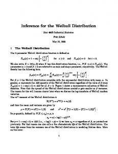
Figure 1: Empirical survival function (bold line) and the fitted survival functions (dotted lines) for Dataset 1 (ZrO2 -TiB2 composite).

1 0.9

Weibull

0.8

Normal

0.7

Empirical

Survival proportions

0.6 0.5 0.4

Log−normal

0.3

Gamma 0.2

Gen. Exp.

0.1 0

4

6

8

10

12

14

16

Strength (MPa units/100)

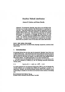
Figure 2: Empirical survival function (bold line) and the fitted survival functions (dotted lines) for Dataset 2 (ZrO2 ceramic).

24

1

Weibull

0.8

Survival proportions

Normal 0.6

Gamma 0.4

Log−normal Gen. Exp.

0.2

0

Empirical

0

2

4

6

8

10

12

14

Strength (MPa units/100)

Figure 3: Empirical survival function (bold line) and the fitted survival functions (dotted lines) for Dataset 3 (Si3 N4 ceramic).

1

Empirical 0.8

Survival proportions

Weibull 0.6

Normal Log−normal 0.4

Gamma Gen. Exp.

0.2

0

0

0.5

1

1.5

2

2.5

3

3.5

4

Strength ((MPa units − 45)/10)

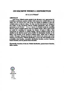
Figure 4: Empirical survival function (bold line) and the fitted survival functions (dotted lines) for Dataset 4 (glass).

25