ISCAS 2000 - IEEE International Symposium on Circuits and Systems, May 28-31, 2000, Geneva, Switzerland
DYNAMIC PROPERTIES OF A MULTIWAY ARBITER Anthony C. Davies Department of Electronic Engineering, King’s College London, Strand, London, WC2R 2LS, England e-mail:
[email protected]
other already-waiting processes having equal or higher priority to the new one). Figure 2 illustrates this for a three-way arbiter.
ABSTRACT A multiway arbiter may be constructed from an interconnected structure of inverting gates which is a generalisation of the bistable flip-flop. Features of the dynamic behaviour of such a ‘multi-flop’ are illustrated by analysis and simulation based on a very simple non-linear dynamic model of each gate. Limitations of such a component as an arbiter are explained.
process 1
request / release
1. INTRODUCTION
shared resource
process 2
process 3
1.1 The Multiflop A symmetric cross-coupled structure of n gates which is a direct generalisation of the bistable flip-flop can be used as a ‘1 out of n’ arbiter to enforce mutual exclusion in distributed and multi-tasking computing systems. Van Berkel and Molnar [1] have pointed out problems of metastability and unfairness associated with the three gate (‘1 out of 3’) structure, illustrating them by a SPICE simulation of realistic CMOS gates. Davies [2] has shown some aspects of the behaviour of these ‘multi-flops’ derived from simulation of a simple gate model. This paper presents a more detailed analysis. u1
x1
u2
x3
u4
grant
Figure 2. Controlling mutually-exclusive access to shared resource The design of two-way arbiters is well established, often based on a bistable flip-flop, with design precautions to minimise the probability of metastability in the case of asynchronous systems. A multi-way arbiter may be made from networks of two-way arbiters, but this results in increased latency in response to requests, and a direct implementation of a multi-way arbiter is attractive. The multi-flop appears to be a solution to this requirement [3].
1.3 Using the Multi-flop as an Arbiter
x2
u3
Tri-flop (arbiter)
x4
Figure 1. Four-flop structure A four-flop based on NAND gates is shown in Figure 1. When all the inputs are held at logic-zero (Vlow), the outputs are all forced to logic-one (Vhigh). If any single input is raised to logic-one, the corresponding output goes to logic-zero. When all inputs are at logic-one, there are n stable states, each one having a single output at logic-zero.
1.2 Requirements of an Arbiter Multi-processing systems typically require access to shared resources or services subject to a restriction that at most one process can have access to a particular resource or service at any time. An arbiter is used for implementing such access control. When any process requests access the arbiter responds by issuing a ‘grant’ signal if the required resource is available. If the resource is busy, the arbiter delays the grant until the release of the resource has been signalled by the process using the resource (and by any
All inputs of the multi-flop are kept at logic-zero (Vlow) while there is no service request, so forcing all outputs to logic-one (Vhigh). Any single input going high (request) forces the corresponding output low (grant). Until the input has returned to low (indicating release of the resource), requests on any other inputs have no effects on any outputs. If there is only one pending request, it is clear that the multi-flop will respond to the release of the first grant by lowering the correct output to grant access to the process which made this pending request. When there is more than one pending request, the behaviour can become rather complicated, as will be seen later on. Simulated behaviour of a four-flop used as an arbiter is shown in Figure 3(a) for four requests with a maximum of one pending request at any time, and in Figure 3(b) for four requests all overlapping in time. It can be seen that the overall response time is significantly delayed in the second case, with irregular waveforms caused by metastability. Note particularly the delayed response to the request on u1. Moreover, the order of responding to the requests does not comply with their order of arrival. The actual order depends on small differences in the parameters of the simulated gates. The busy period (the time for which each process uses the resource) was made equal for each case.
0-7803-5482-6/99/$10.00 ©2000 IEEE
III-221
3. SMALL-SIGNAL LINEAR ANALYSIS
2. MODELLING AND SIMULATION 2.1 First-order Gate model
3.1 Dynamics around m
Many aspects of the dynamic behaviour may be illustrated with very simple gate models. Figure 4 shows the NAND gate model used, comprising a cascade of a minimum-selector, the non-linear transfer characteristic, and a linear first-order low-pass filter.
The conventional procedure for small-signal analysis is to linearise around some operating point. However, although a piecewise-linear model is being used, investigating the behaviour of an n-flop with n > 2 around m is complicated because the ‘minimum’ function partitions the regions around m into n! linear segments, all meeting on the line between the (000..0) and (111..1) vertices, passing through m. This results in a non-linearity exactly at m. Any deviation from m places the operation in one of these n! segments. For the three-flop, the six segments are defined by: Sijk = [xi > xj > xk, {i, j, k} ∈ {1,2,3}, i ≠ j ≠ k] Denoting deviations from m by ε: xi = m + εi for each i the state-equations for small deviations from m while all inputs are high are then: x2 , x3 ε 1 −1 0 0 ε 1 d ε 2 = 0 − 1 0 ε 2 − g min x1 , x3 dt x1 , x2 ε 3 0 0 − 1 ε 3
out
min
F:
F
R
in
C
x
Figure 4. First-order model of NAND gate
2.2 Multiflop State-equations One first-order differential equation is needed for each gate, and the equations for a four-flop are as follows. F is the non-linear transfer characteristic of the gate, τ is the gate time-constant and the gate outputs are the state-variables.
(
dx1 1 = − x1 + F1[ min( x2 , x3 , x4 , u1 ) ] dt τ1
)
(
)
(
)
(
)
dx2 1 = − x2 + F2 [ min( x1 , x3 , x4 , u2 )] dt τ2 dx3 1 = − x3 + F3 [ min( x1 , x2 , x4 , u3 )] dt τ3
dx4 1 = − x4 + F4 [ min( x1 , x2 , x3 , u4 )] dt τ4 For algebraic simplicity is convenient to normalise F so that the digital signal levels are 0V and 1V. This makes the state-space a hypercube with vertex coordinates at (0,1). No trajectory can go outside this hypercube.
2.3 Metastable points The metastable point, m, is an unstable fixed-point defined by:
[
xi = Fi min( x j , j = 1.. n, i ≠ j )
Thus, for the 4-flop:
]
−g is the slope of F at m. For simplicity of description it will be assumed that the deviations are all positive, so that the state variables in the ‘minimum’ function can be replaced by deviations. (When this is not the case, the analysis method is the same.) The equations then become: d ε =− I ε − gTε = Aε dt where T is a matrix containing n ‘ones’ which selects the appropriate elements of ε for the particular one of the n! different segments into which the deviation from m takes the state. If j is the index of the smallest state-variable, and k is the index of the smallest but one, then T has a ‘one’ in column j of every row except j, and a ‘one’ in column k of row j. All other elements (including the diagonal) are zero. The simple equation structure enables the eigenvalues to be easily determined:
sI−A = ( s + 1) n − 2 ( s + 1 − g )( s + 1 + g ) The eigenvalues do not depend upon the choice of T, and it can be seen that there is always one real positive eigenvalue whenever g > 1, and all other eigenvalues are real and negative. This is to be expected, and shows that trajectories always move away from m. The eigenvectors, which determine the direction of the trajectory, do depend on T.
x1 = F1[ min( x2 , x3 , x4 )]
x2 = F2 [ min( x1 , x3 , x4 )] x3 = F3[ min( x1 , x2 , x4 )]
x4 = F4 [ min( x1 , x2 , x3 )] If the Fi are all identical and such that input and output voltages are equal at 0⋅5V, the ‘metastable’ point, m, is at the centre of the hypercube. m = (m,m,m,...m) m = 0⋅5 Trajectories typically move very slowly in the vicinity of m which results in sluggish response and often can lead to system maloperation. Because the tri-flop has a state-space of only three dimensions, its dynamic behaviour can be illustrated by means of perspective representations in two dimensions of the trajectories in this statespace.
Since A = − I − gT and A = QΛQ −1
Λ + I = − gQ −1TQ For the three-flop in a segment where x1 > x2 > x3, 1 1 1 0 0 1 T = 0 0 1 and Q = 0 1 1 0 − 1 1 0 1 0 In the case of the other segments, the elements of Q have the same values, but in different locations. For a more specific illustration of the transient leading away from the vicinity of m, suppose g = 5 and assume an initial state x = [m+3d, m+2d, m+d]T where d is a small deviation.
III-222
1 1 1 ε(t ) = J 0 exp( − t ) + K 1 exp(4t ) + L 1 exp( −6t ) 1 −1 0
3.3 Second-order Gate model
Solving for the constants J, K, L, 3d / 2 d / 2 d ε(t ) = 0 exp( −t ) + d / 2 exp(4t ) + 3d / 2 exp( −6t ) 3d / 2 − d / 2 0
As t increases, the second term dominates, so that 0.5 d / 2 x(t ) = m + ε ( t ) ≈ 0.5 + d / 2 exp(4t ) 0.5 −d / 2
The trajectory moves at an exponentially increasing rate and heads for the (1,1,0) vertex. Differing initial deviations lead to the other (stable) vertices (0,1,1), (1,0,1). When the initial deviation is very small, the initial movement is very slow (e.g. the state-variables remain near m for a significant time) which is the well-known symptom of metastability. The first order gate model was used for the simulations of Figure 3, and the above small-signal analysis is sufficient to explain the waveforms and the metastability observed in Figure 3(b).
3.2 Trajectories towards m Since for a NAND gate F(Vlow) = Vhigh, whenever the statevariables are all near zero the state-equations simplify to: dxi 1 = − xi + Vhigh for i = 1,2,... n dt τ i The equations are de-coupled and each gate output increases towards Vhigh, approaching m as it does so. Since m is an unstable fixed point, the trajectory deviates away from m, and if the inputs to the multi-flop are all high, finally terminates on one of the stable vertices by means of the mechanism described in Section 3.1. This is illustrated by Figure 5. In the case that the inputs are all low, it continues past m and terminates on the (111..1) vertex.
(
)
The first-order model of Figure 4 gives only real eigenvalues, ensuring that all transients are exponentials, with no overshoot or oscillation in the trajectories. By associating an additional time constant with the gate-input (following the ‘minimum’ function), the possibility of complex eigenvalues may be modelled, and overshoot observed in the simulation. This doubles the number of state equations, but there is no significant change to the procedure. If all time constants are equal, it is easy to see that the six eigenvalues of the three-flop are: −1, −1, −(1 + √g), −1 ± j√g, √g − 1 so there is the expected real RHP eigenvalue when g > 1 and a pair of complex LHP eigenvalues, the imaginary part of which increases with increase in g. Thus not only the trajectory speed but also the frequency of any damped oscillation within it increases with g. This gives a qualitative indication of the behaviour to be expected in transients around the metastable point.
4. CONCURRENT REQUESTS 4.1 Stable states of n-flop There are no stable equilibrium states with two or more outputs low, whatever the inputs. If there are (n−2) zeros in the input pattern, just two gates are left whose outputs are not directly forced high, which form a conventional bistable latch - with two stable states when both inputs are high. Similarly, (n−3) input zeros create a subsystem of three gates, forming a tri-flop which, with all inputs high, has three stable states, each with a single low output. In general, for (n−r) zeros, there is an r-flop subsystem with r stable states when all its inputs are high.
4.2 Other metastable points Suppose that there are p concurrent requests to an n-flop (p ≤ n). (n − p) inputs remain low, forcing the corresponding gate outputs high, and so these gates have no influence on the dynamic behaviour of the rest of the n-flop. The study of the response to these p requests therefore requires an understanding of the behaviour of a p-flop, the p-dimensional state-space of which is a p-dimensional hypercube, having its metastable point at its centre. The metastable points of this p-flop are defined as for the n-flop (see Section 2.3) - e.g. by deleting the (n − p) state-variables which remain high, as set of p non-linear equations remain which define the metastable point of this situation. Thus, for a four-flop with three concurrent requests, the trajectories move within a 3-cube, and may involve metastability around the centre of this 3-cube. When there are only two concurrent requests, the trajectories remain on a face of a 3-cube, with a metastable point at the centre of the face (this is therefore identical dynamics to the conventional bistable flip-flop).
Figure 5. Trajectory from origin via m to a stable fixed point
Figure 6 illustrates a trajectory resulting from three simultaneous requests to a tri-flop. The tri-flop grants access to process 3 after a close approach to the metastable point, m, in the centre of the cube (denoted m3) then grants access to process 2 after approaching a metastable point (denoted m2) on a face of the cube. Finally, a
III-223
normal transient leads to the grant of access to process 1 then return of the tri-flop to the rest state.
5. DISCUSSION AND CONCLUSIONS In most systems, metastability is infrequent and seldom-observed. In the case of the multi-flop used as an arbiter, metastable responses can be expected whenever there are several pending requests held by the arbiter. At the moment of release of a previously-accepted request, the simultaneous activation of the pending requests typically results in a metastable transient, from which the winner depends not at all on the sequence of arrival of the pending requests, but on normally-small differences in the parameters of the nominally-identical gates forming the multi-flop. Despite its simplicity and short latency, the multi-flop structure cannot be recommended without reservations as an arbiter because of this likelihood of metastability and inability to maintain sequentiality in the responses to concurrent requests. However, its dynamic behaviour shows interesting characteristics, many of which can be revealed by study and simulation of simple piecewise-linear models, and it is an interesting structure in its own right.
Figure 6. Tri-flop trajectory from 3 simultaneous requests
4.3 Overlapping Requests and Unfair Arbitration If more than one request occurs before the first grant has been released, the sequence of granting the subsequent requests may be interchanged, and, as illustrated in Figure 3, metastable transients are likely. This is because, at the instant of releasing the first grant, the other gates have their inputs simultaneously raised to Vhigh while their outputs are already at Vhigh. This is a symmetrical situation for these gates, and the precedence of the pending requests is lost. While inputs are rising and outputs falling, the trajectory moves into the cube interior, sometimes very close to m, then diverges towards one or other stable state, the selection of which depends upon detailed differences in characteristics of the gates rather than on the sequence of arrival of requests. For gates with very similar time-constants and non-linear transfer characteristics, this trajectory closely approaches m, resulting in a longer metastable transient than if the gates are dissimilar. A fair arbiter could be expected to allocate the shared resource to the requesting processes in the same sequence as the requests are made (assuming all requests are of the same priority level) [4]. The multi-flop clearly does not do this.
Acknowledgements: The U.K. Engineering and Physical Sciences Research Council is thanked for financial support (Grant No. GR/L92471), and colleagues at King’s College London and the University of Newcastle-upon-Tyne for interesting discussions.
6. REFERENCES [1] C.H. van Berkel and C.E. Molnar ‘Beware the 3-way arbiter’, IEEE Journal on Solid-state Circuits, vol. 34, pages 840-848, 1999 [2] A.C. Davies ‘Multi-flops - a view of the dynamic behaviour’ Proc. NDES’99, 15-17 July 1999, Rønne, Bornholm, Denmark, pages 133-136. [3] D.J. Kinniment, A. Yakovlev and B. Gao ‘Metastable behaviour and system performance’ Prof. 2nd UK Forum on Asynchronous Systems, Department of Computing Science, University of Newcastle upon Tyne, July 1997 [4] A. Bystrov and A. Yakovlev ‘Ordered Arbiters’ Electronics Letters, vol 35, pages 877-879, 1999
Figure 3(b). “metastable behaviour” of 4-flop arbiter: response to four concurrent requests at 65, 55, 60, 50. (some granted out of sequence)
Figure 3(a). “correct behaviour” of 4-flop arbiter: response to four requests at 50, 300, 550, 800.
III-224