1
iSeg: an algorithm for segmentation of genomic data
arXiv:1506.08334v1 [stat.AP] 27 Jun 2015
S.B. Girimurugan1¶∗ , Jonathan Dennis2& , Jinfeng Zhang3¶∗ 1 Department of Mathematics, Florida Gulf Coast University, Fort Myers, FL, USA 2 Department of Biological Science, Florida State University, Tallahassee, FL, USA 3 Depart1ent of Statistics, Florida State University, Tallahassee, FL, USA ∗ E-mail:
[email protected] ¶ These authors contributed equally to this work. & This author also contributed equally to this work.
Abstract Identification of functional elements of a genome often requires dividing a sequence of measurements along a genome into segments differing from adjacent segments. In many applications, the mean of the measured values at multiple genomic locations in a segment is used to make inference of the property of interest. The segments with non-zero means often correspond to genomic regions with certain biological events, such as changes between two conditions. This problem is often called the segmentation problem in the field of genomics, and the change-point problem in other scientific disciplines. We designed an efficient algorithm, called iSeg, for segmentation of high-throughput genomic profiles. iSeg first utilizes dynamic programming to compute the significance for a large number of candidate segments. It then uses tree-based data structures to detect overlapping significant regions and update them simultaneously. Refinement and merging of significant segments are performed at the end to generate the final segmentation. We evaluate iSeg using both simulated and experimental datasets and show that it performs quite well when compared with existing methods.
Introduction High throughput experiments, such as microarray and sequencing, are powerful tools for studying genetic and epigenetic functional elements at genome scale [1]. There has been a large number of studies on the analysis of gene expression data generated from high-throughput experiments [2]. When measuring gene expressions, the genomic locations of genes are known and multiple probes (or short reads) can be mapped to a gene to obtain its expression values. With replicates from two experimental conditions, standard hypothesis tests, such as t-test, can be performed to infer the differentially expressed genes. On the other hand, the situation is quite different for functional elements without predefined locations (i.e. starting and ending positions). Consider DNA copy number as an example. When detecting the changes in DNA copy number between two experimental conditions, one needs to consider a very large number of regions that can possibly undergo changes. The number is usually much larger than the total number of genes. Other functional elements especially epigenetic features fall into the same category. This poses a significant challenge to the analysis of such type of data. The problem is usually formulated as segmenting a sequence of measurements along the genome. For example, if segments without changes have a mean value of zero and those with changes have nonzero
2 means, then the goal is to identify those segments of the genome whose means are significantly above or below zero. A number of methods have been developed recently and many of those were tested on analysis of DNA copy number variations (CNVs) for microarray-based comparative genomic hybridization (aCGH) data [3–15]. The previous methods fall into several categories including change-point detection [3, 5, 8– 10, 12, 16–23], Hidden Markov models [11, 15, 24–26], Dynamic Bayesian Network (DBN) models [27, 28], signal smoothing [29–32], and variational models [33, 34]. For review and comprehensive comparison, please refer to [35–38]. In recent years, many efforts have been focused on developing methods for segmentation of multiple profiles simultaneously [7, 39–51]. Despite significant progresses made in this area, further improvement in terms of both accuracy and computational speed is still desirable. In addition, some methods require users to adjust parameters to obtain acceptable results. In this study, we designed an algorithm to segment genome-wide profiles to achieve better accuracy and efficiency compared to existing methods. In addition, we minimize the number of parameters users have to tune so that our method can be easily applied by biologists with limited analytical expertise. Our method, iSeg (implemented in C++), has shown superior performance on both simulated data and benchmark experimental data compared with previous methods. The next section describes the method in detail.
Materials and Methods Most segmentation methods have an underlying assumption of normality. For instance, the test statistics in [3, 10, 13] are modified versions of a t-statistic. We make a similar assumption in this study, so the comparison with existing methods is straightforward. Consider a sample consisting of N measurements along the genome in a sequential order, X1 , X2 , . . . , XN , and Xk Xk
∼
∼
N (0, σ 2 ), N (µi , σ 2 ),
∀k ∈ G
∀k 6∈ G
(1) (2)
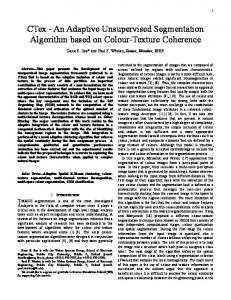
for some set of locations ‘G’. The common assumption is that there are M non-overlapping segments with mean µ1 , µ2 , . . . , µi , . . . , µM , where µi 6= 0, and the union of these segments will form the complement of the set ‘G’. If the background level is non-zero, tests can be performed over segments for this level instead of testing against zero. According to this model, it is possible for multiple segments with different non-zero means to be adjacent to each other. In addition, all the measurements are assumed to be independent. This assumption has been employed in many existing methods [3, 17]. A summary of existing methods that use such an i.i.d assumption and its properties are nicely discussed in [52]. The goal of a segmentation method is to detect all the M segments with non-zero means. A formal description of change-point problems is given in [53]. As an example, (Fig. 1(A)) shows segments sampled from Normal distributions with non-zero means where the rest of the data is sampled from a standard Normal distribution. One approach used by some of the previous methods [3, 13] is to first find a segment with the highest significance (or smallest p-value), remove the segment and repeat the process for the rest of the profile until all the segments with significance higher than a threshold value are identified. There are two computational challenges associated with this approach that also manifest in many previous methods. First, the number of segments that have to be examined is very large; Second, the overlaps among significant segments need to be detected so that the significance of the overlapping segments can be adjusted accordingly. To deal with the first challenge, we applied dynamic programming combined with exponentially increased segment scales to speed up the scanning of a large sequence of data points. The resulting optimization approach is top-down with memoized computations identifying optimal substructures. To deal with the second challenge, we designed an algorithm coupling two balanced binary trees to quickly detect overlaps and update the list of most significant segments. Segment refinement and merging allow iSeg to detect segments of arbitrary length. The details of the
3
Figure 1. One of the simulated profiles and its detected segments obtained using iSeg. (A) The actual data with background noise and meaningful segments. The segments with non-zero means are normally distributed with unit variance and means 0.72, 0.83, 0.76, 0.9, 0.7, and 0.6 respectively. The profiles shown here are normalized for an approximate signal to noise ratio of 1.0. The segments detected by iSeg (B) and other existing methods: snapCGH (C), mBPCR (D), cghseg (E), cghFLasso (F), HMMSeg (G), DNAcopy (H) and fastseg (2) Comparison of F1 -scores for the simulation profiles with SNR≃1.0. Since the profiles are simulated, the SNR of the resultant profiles is approximately one. The SNR defined during the simulation is exactly one.
4 algorithm are given below.
Computing p-values using dynamic programming iSeg scans a large number of segments starting with a minimum window length, Wmin , and up to a maximum window length, Wmax . They have default values 1 and 300, respectively. This window length increases by a fixed multiplicative factor, called power factor (ρ), with every iteration. For example, the shortest window length is Wmin , and the next shortest window length would be ρWmin . The default value for ρ is 1.1. When scanning with a particular window length, W, we use overlapping windows with a space of W/5. When ‘W’ isn’t a multiple of 5, numerical rounding (ceil) is applied. The aforementioned parameters can be changed by a user. The algorithm computes p-values for candidate segments and detects a set of non-overlapping segments most significant among all possible segments. Given the normality assumption, a standard test for mean is the one-sample student’s t-test, which is commonly found among many existing methods. The test statistic for this test is, √ x ¯ n t = (3) s where x¯ is the sample mean, s is the sample standard deviation, and n is the sample size. A drawback of this statistic is that it cannot evaluate segments of length 1. This may be the reason that some of the previous methods are not good at detecting segments of length 1. Although we can derive a test statistic separately for segments of length 1, the two statistics may not be consistent. To solve this issue, we first estimate the sample standard deviation using median absolute deviation and assume that the standard deviation is known. This allows us to use z statistic instead of t statistic and the significance of single points can be evaluated based on the same model assumption as longer segments. To calculate sample means for all segments to be considered for significance, the number of operations required by a brute force approach is ‘Cb ’. Cb
=
k X i=0
(N − ρi Wmin )ρi Wmin
(4)
where, ρk Wmin ≤ Wmax and ρk+1 Wmin > Wmax . Computation of these parameters (means and standard deviations) for larger segments can be made more efficient by using the means computed for shorter segments (top-down memoization of dynamic programming). For example,the running sum of a shorter segment of length ‘m’ given by, Sm =
m X
Xi ,
(5)
i=1
If this sum is retained, the running sum of a longer segment of length ‘r’(> m) in the next iteration can be obtained as, Sr = Sm +
r X
Xi
(6)
i=(m+1)
and the means for all the segments can be computed using these running sums. Now, the total number of operations (Cb∗ ) is Cb∗
= N+
k X i=0
(N − ρi Wmin )
(7)
5 which is much smaller in practice than the number of operations (Cb ) without using dynamic programming. Computation of standard deviations are sped up using a similar memoization process resulting in computational efficiency.
Detecting overlapping segments and updating significant segments using balanced binary trees When the p-values of all the segments are computed, we rank the segments by their p-values from smallest to largest. All the segments with p-values smaller than a threshold value, ps , are kept in a balanced binary tree (BBT1). We set ps as 0.001 in this study to speed up the computation. With thousands of hypothesis tests being performed usually for a particular dataset, this cutoff is reasonable. Assuming a significance level (α) of 0.1, 100 simultaneous tests will maintain a family-wise error rate (FWER) bounded by 0.001 with Bonferroni and Sidak corrections. Thus, the cut-off is an acceptable upper bound for multiple testing. It can be changed by a user if necessary. The procedure is described below as a pseudo-code. The set SS stores all significant segments. The second balanced binary tree (BBT2) stores the boundaries for significant segments. After the procedure, SS contains all the detected significant segments. The selection of segments using balanced binary tree aims to minimize the p-values for individual segments. When the minimization causes some segments to overlap, the one with smaller p-value is selected. procedure SelectSignificantSegments initialize BBT2 // BBT2 is empty at the beginning while(BBT1 not empty) S = top ranked segment in BBT1 (smallest p-value among all segments in BBT1) delete S from BBT1 l = left boundary of S r= right boundary of S if(checkoverlap (BBT2, l, r) == FALSE) // no overlapping insert pair(l, r) into BBT2 insert S to set SS
Refinement of significant segments The significant segments are refined further by expansion and shrinkage. Without loss of generality, in the procedure (see SegmentExpansion text box) we describe expansion on left side of a segment only. Expansion on the right side and shrinkage are done similarly. When performing said expansion and shrinkage, a condition to check for overlapping segments is applied so the algorithm results in only disjoint segments.
6
Merging adjacent significant segments When all the significant non-overlapping segments are detected and refined in the previous steps, iSeg performs a final merging step to merge adjacent segments. The procedure is straightforward. We check each pair of adjacent segments. If the merged segment, whose range is defined by the left boundary of the first segment and the right boundary of the second segments, has a p-value smaller than those of individual segments, then we merge the two segments. The new segment will then be tested for merging with its adjacent segments iteratively. The procedure continues until no segments can be merged. Apart from refinement, merging also prevents partitioning of a signal into only short segments. Short segments are called significant only if a longer segment or several merged segments are insignificant. With refinement and merging, iSeg can detect segments of arbitrary length— long and short. procedure SegmentExpansion (Sl,r ) /* Sl,r : the segment to be expanded. Its left boundary is l, and right boundary is r. */ S = Sl,r while() p = p-value of S L = length of S l0 = left boundary of S /* expand the segment by 1/K of its current length, and compute its p-value. The default value for K is 10. */ l′ = l0 − ceiling(L/K) p′ = p-value of segment Sl′ ,r if p′ < p S = Sl′ ,r else compute p-values for all segments with left boundary in (l′ , l0 ) and right boundary r. let pm be the minimum p-value of these segments, and lm be the corresponding left boundary if pm < p S = Slm ,r break Update Sl,r with boundaries of S.
Multiple comparison In iSeg, p-values for potentially significant segments are calculated. Using a common p-value cutoff, for example 0.05, to determine significant segments can suffer from a large number of false positives due to multiple comparison. To cope with the multiple comparison issue which can be very serious when the sequence of measurements is long, we use a false discovery rate (FDR) control. Specifically, we employ the Benjamini-Hochberg (B-H) procedure [54] to obtain a cutoff value for a predefined false discovery rate (α), which has a default value of 0.01, and can also be set by a user. Other types of cutoff values can be used to select significant segments, such as a fixed number of most significant segments.
Biological cutoff Often in practice, biologists prefer to call signals above a certain threshold. For example, in gene expression analysis, a minimum of two-fold change may be applied to call differentially expressed genes. Here we add a parameter, pb , which can be tuned by a user to allow more flexible and accurate calling of significant segments. Such a cutoff is quite useful in situations where the baseline is non-zero.
7
Results We compare our method with several previous methods for which we can obtain executable programs: HMMSeg [55], CGHSeg [12], DNAcopy [3, 16], fastseg [10], cghFLasso [31], BioHMM-snapCGH [24] and mBPCR [5]. Each method has some parameters that can be tuned by a user to achieve better performance. In our comparative study, we carefully chose the parameters based on the recommendations provided by the authors of such methods. For each method, a single set of parameters is used for all data sets. Post-processing is required by some of the methods to identify significant segments. In our analysis, performance is measured using F1 -scores [56] for all methods. F1 -scores are considered as a robust measure for classifiers, as they account for both precision and recall in their measurement. The F1 -score is defined as, F1 = (2pr)/(p+r)
(8)
where p is precision and r is recall for a classifier. In terms of the true and false positives, p = r =
T P/(T P +F P ) T P/(T P +F N ).
(9) (10)
Since an effective threshold is not varied to assess performance in the space of sensitivity and specificity, our analysis implements F1 -scores. These scores have been shown to effectively assess the performance of various classifiers (including support vector machines) and are claimed as viable alternatives to approaches such as ROC, AUC etc. [57]. The methods CGHSeg, DNAcopy, and fastseg depend on random seeds given by a user (or at run-time automatically), and the F1 -scores at different runs are not the same albeit very close. These methods were run using three different random seeds, and the averages of the F1 -scores were used to measure their performance. In the following sections, we assess iSeg’s performance using both simulated data and experimental benchmark data.
Performance on simulated data The simulation profiles were generated under varying noise conditions, with signal to noise ratios (SNR) of 0.5, 1.0 and 2.0, which correspond to poor, realistic and ideal cases. Ten different profiles of length 5000 are simulated. For each profile, five different segments of varying lengths are predefined at different locations. Data points outside of these segments are generated from normal distribution with mean zero. The five segments are simulated with non-zero means and varying amplitudes (some easy to detect and some rather difficult) in order to assess the robustness of the methods. (Fig. 1) shows an example of the simulated data and the segments identified by iSeg and other existing methods. (Fig. 2(A)) shows the performance of iSeg and other methods on simulated data with SNR = 1.0. We can see that iSeg, DNACopy and CGHSeg perform similarly well, with HMM and CGHFLasso performing a little worse while fastseg did not perform as well as the other methods. iSeg is also tested using a set of 10 longer simulated profile, each of length 100000. Seven segments are introduced at varying locations along the profiles. iSeg performs still quite well in these very long profiles. The performance of these methods on long sequences is shown in (Fig. 2(B)).
Performance on experimental data To assess the performance of iSeg on experimental data, we use three different datasets: 11 profiles from [58], called Coriell dataset; three profiles from [59] , called BACarray dataset; and two profiles
8
Figure 2. Comparison of F1 −scores of various methods in analyzing different types of profiles. A. Simulated Profiles B. Simulated Long Profiles (n=100K) C. Coriell (Snijders et al.) Profiles D. BACarray Profiles taken from TCGA (The Cancer Genome Atlas), called TCGA dataset. The 11 profiles in Coriell datasets correspond to 11 cell lines: GM03563, GM05296, GM01750, GM03134, GM13330, GM01535, GM07081, GM13031, GM01524, S0034 and S1514. We construct “gold standard” annotations using a consensus approach. We first run all the methods using several different parameter settings for each method. The resulting segments are evaluated using the test statistic described in this method. The set of gold standard segments are obtained using Benjamini-Hochberg procedure to account for multiple comparisons. The annotations derived using a consensus approach are provided as Supplementary material. The 11 profiles from the Coriell dataset were segmented using iSeg and the other methods, and the F1 -scores are shown in (Fig. 2(C)) The performance of iSeg is robust with accuracy above 0.75 for all the profiles from this dataset and it is comparable to, better in some cases, other methods. For HMMSeg, both no-smoothing and smoothing are used. The best smoothing scale for HMMSeg was found to be 2 for the Coriell dataset. The segmentation results for one profile in Coriell dataset is shown in (Fig. 3). We can see that iSeg identified most of the segments. While DNAcopy, fastseg, HMMSeg and cghseg missed single-point peaks, cghFLasso, mBPCR and snapCGH missed some longer segments. The segmentation results for other profiles in Coriell dataset can also be found in the Supplementary material. We generated annotations using the consensus method for BACarray dataset similar to the Coriell dataset. The comparison of F1-scores is shown in (Fig. 2(D)) and the comparison of segmentation results is shown in (Fig. 4). iSeg has better F1 -scores than the other methods and a similar conclusion can also be gathered from visual inspection. For TCGA datasets, since the profiles are rather long, we did not generate annotations using the consensus approach. We apply some of the methods on this dataset and compared their segmentation results (Fig. 5). Again, we can see that iSeg identified most of the significant peaks. DNACopy performs well overall, but tends to miss single-point peaks while other methods did not perform as expected. We compare the computational time of iSeg with those of the other methods. Table 1 shows that iSeg is the fastest method for all three data sets. It is worth noting that for very long profiles (length 100000),
9
Figure 3. Comparison of segmentation results obtained for the Coriell dataset. (A) The gold standard segmentation obtained using a consensus approach. Segmentation results of iSeg (B) and other existing methods: snapCGH (C), mBPCR (D), cghseg (E), cghFLasso (F), HMMSeg (G), DNAcopy (H) and fastseg (I).
Figure 4. Comparison of segmentations for BACarray dataset. (A) The gold standard segmentation obtained using a consensus approach for the TCGA Glioblastoma Multiforme (GBM) profile. Segmentation results of iSeg (B) and other existing methods: snapCGH (C), mBPCR (D), cghseg (E), cghFLasso (F), HMMSeg (G), DNAcopy (H) and fastseg (I).
10
Figure 5. Comparison of segmentations for the TCGA dataset. The patient profile ID is TCGA-02-0007 and the data is supplied by the Harvard Medical School 244 Array CGH experiment (HMS). Segmentation results of iSeg (A) and other existing methods: DNAcopy (B), cghFLasso (C), and cghseg (D). The peaks pointed by the arrows and the region labeled by the red, and green squares are identified by iSeg, but not all of them are detected by the other three methods. Overall, iSeg consistently identifies all the significant peaks. Other methods often miss peaks or regions which are more significant than those identified. iSeg takes much less time than the other methods. The use of dynamic programming and a power factor makes the initial scanning of a profile fairly fast. The long profiles contain similar amount of data points that are signals (as opposed to background or noise) as the shorter profiles. The time spent on dealing with potentially significant segments is roughly the same between the two types of profiles. As a result, the overall running time of iSeg for the long profiles does not increase so much as the other methods. In summary, iSeg runs faster than the other methods, and much faster for profiles with sparse signals.
Discussion In this study, we designed an efficient method, iSeg, for the segmentation of large-scale genomic profiles. When compared with existing methods using both simulated and experimental data, iSeg shows superior accuracy and speed. iSeg performs equally well when tested on very long profiles, making it suitable for real-time, online applications involving large-scale genomic datasets. In this study, we have assumed that the data follow a normal distribution. The algorithm is not limited to this distribution and other hypothesis tests can be used to compute p-values for the segments. It has been shown that data generated by next-generation sequencing (NGS), which has gained much popularity in genomics research, may follow a Poisson or a negative binomial distribution [60,61]. We aim to implement these two distributions
11 in the near future. The use of dynamic programming and a power factor makes iSeg computationally more efficient when analyzing very long profiles, especially with sparse signals as noted in many NGS data sets. The refinement step identifies the exact boundaries of segments found by the scanning step. Merging allows iSeg to detect segments of any length. Together, these steps make iSeg an accurate and efficient method for segmentation of sequential data. Methods such as VEGA [62] isolate segments while accounting for serial dependence using a piece-wise smoothing model and minimization of a cost function. However, a piece-wise smoothing model could be problematic especially in the presence of sharp changes (peaks or very narrow segments) on a short interval. Such a method could miss short segments by calling a longer segment containing the short segment. This behavior could be seen in some results shown in [62] when comparing to Ultrasome [63] and SMAP [64]. iSeg overcomes such issues retaining a narrow segment, or a peak, if it is deemed significant.Although tested only on DNA copy number data, in principle, iSeg can be used to segment other types of genomic data, such as DNA methylation and histone modifications. Some adaptation or parameter tuning may be needed for different data types. The statistic used in our method is very similar to the one used in [13], which is based on similar model assumptions as some of the previous methods. However in [13], the segments are identified using an exhaustive approach, which will not be efficient when the profiles to be segmented are very long. To speed up computation, the method in [13] assumes that the segments have relatively short length, which is not true for some datasets. The algorithm designed in this study allows us to detect segments of any length with greater efficiency. The gold standard generated using the consensus approach does not guarantee that the true optimal segments will be identified. In addition, the F1 -scores may favor iSeg more as the test statistic used to generate the gold standard is not employed by the other methods. However, the statistic we used is based on model assumptions used by many existing methods and can be used in evaluating segments of length 1 or more. Some existing test statistics cannot be used for segments of length 1, which is the reason why they tend to miss such segments. Clearly, visual inspection of segmentation results shows that iSeg performs better than the other methods in this study. A natural extension of iSeg will be to compare multiple profiles simultaneously. This will be a subject for our future research. We have designed the method to make it flexible and versatile. This resulted in a number of parameters that users can tune. However, the default values work well for all the simulated and experimental datasets. In practice, to obtain satisfactory results, users are not expected to modify any parameters. The speed of iSeg would allow us and fellow researchers to implement it as an online tool to deliver segmentation results in real-time.
12
Tables Table 1. Comparison of computational times (in seconds) on simulated data and Coriell data. Method
Simulation (SNR≃1.0, n=5000)
Simulation (SNR≃1.0, n=100K)
iSeg (C++) 0.164 1.223 DNAcopy (R) 2.267 60.343 fastseg (R) 0.647 48.139 CGHSeg (R) 54.480 157.626 HMMSeg (Java) 0.543 160.790 Table 2. The table summarizes total computational times required Coriell profiles.
Coriell 0.294 3.098 0.630 24.36 0.552 to process 10 simulated and 11
References 1. Consortium EP, et al. (2012) An integrated encyclopedia of DNA elements in the human genome. Nature 489: 5774. 2. Khatri P, Sirota M, Butte AJ (2012) Ten Years of Pathway Analysis: Current Approaches and Outstanding Challenges. PLoS Computational Biology 8. 3. Olshen AB, Venkatraman ES, Lucito R, Wigler M (2004) Circular binary segmentation for the analysis of array-based DNA copy number data. Biostatistics 5: 55772. 4. Picard F, Robin S, Lebarbier E, Daudin JJ (2007) A Segmentation/Clustering Model for the Analysis of Array CGH Data. Biometrics 63: 758766. 5. Rancoita P, Hutter M, Bertoni F, Kwee I (2009) Bayesian DNA copy number analysis. BMC bioinformatics 10: 10. 6. Zhang NR, Siegmund DO (2007) A modified bayes information criterion with applications to the analysis of comparative genomic hybridization data. Biometrics 63: 2232. 7. Diskin SJ, Eck T, Greshock J, Mosse YP, Naylor T, et al. (2006) STAC: A method for testing the significance of DNA copy number aberrations across multiple array-CGH experiments. GENOME RESEARCH 16: 11491158. 8. Venkatraman ES, Olshen AB (2007) A faster circular binary segmentation algorithm for the analysis of array CGH data. Bioinformatics 23: 65763. 9. Baldi P, Brunak S (1998). The machine learning approach. 10. Baldi P, Long AD (2001) A Bayesian framework for the analysis of microarray expression data: regularized t -test and statistical inferences of gene changes. Bioinformatics 17: 509519. 11. Day N (2007). HMMSeg. URL http://noble.gs.washington.edu/proj/hmmseg.
13 12. Picard F, Lebarbier E, Budinsk E, Robin S (2011) Joint segmentation of multivariate Gaussian processes using mixed linear models. Computational Statistics & Data Analysis 55: 11601170. 13. Jeng XJ, Cai TT, Li H (2010) Optimal sparse segment identification with application in copy number variation analysis. Journal of the American Statistical Association 105: 11561166. 14. Cai T, Jeng J, Li H (2012) Robust detection and identification of sparse segments in ultra-high dimensional data. Journal of the Royal Statistical Society Series B*: 773797. 15. Wang K, Li M, Hadley D, Liu R, Glessner J, et al. (2007) PennCNV: an integrated hidden Markov model designed for high-resolution copy number variation detection in whole-genome SNP genotyping data. Genome research 17: 16651674. 16. Sen A, MS S (1975) On tests for detecting change in mean. The Annals of Statistics 3: 98108. 17. Picard F, Robin S, Lavielle M, Vaisse C, Daudin J (2005) A statistical approach for array cgh data analysis. BMC Bioinformatics 6: 27. 18. Chen J, Wang YP (2009) A statistical change point model approach for the detection of dna copy number variations in array cgh data. Computational Biology and Bioinformatics, IEEE/ACM Transactions on 6: 529541. 19. Chen J, Yiiter A, Chang KC (2011) A bayesian approach to inference about a change point model with application to dna copy number experimental data. Journal of Applied Statistics 38: 18991913. 20. Niu Y, Zhang H (2012) The screening and ranking algorithm to detect dna copy number variations. Annals of Applied Statistics 6: 13061326. 21. YAO Q (1993) TESTS FOR CHANGE-POINTS WITH EPIDEMIC ALTERNATIVES. BIOMETRIKA 80: 179191. 22. Killick R, Eckley IA (2011) Changepoint: an r package for changepoint analysis. R package version 06, URL http://CRAN R-project org/package= changepoint . 23. Cleynen A, Koskas M, Lebarbier E, Rigaill G, Robin S (2013) Segmentor3isback: an r package for the fast and exact segmentation of seq-data. In: The R User Conference, University of Castilla-La Mancha, Albacete, Spain. 24. Marioni JC, Thorne NP, Tavar S (2006) Biohmm: a heterogeneous hidden markov model for segmenting array cgh data. Bioinformatics 22: 11441146. 25. Stjernqvist S, Rydn T, Skld M, Staaf J (2007) Continuous-index hidden markov modelling of array cgh copy number data. Bioinformatics 23: 10061014. 26. Jaschek R, Tanay A (2009) Spatial clustering of multivariate genomic and epigenomic information. In: Research in Computational Molecular Biology. Springer, p. 170183. 27. Hoffman MM, Buske OJ, Wang J, Weng Z, Bilmes JA, et al. (2012) Unsupervised pattern discovery in human chromatin structure through genomic segmentation. Nature methods 9: 473476. 28. Hoffman MM, Ernst J, Wilder SP, Kundaje A, Harris RS, et al. (2012) Integrative annotation of chromatin elements from ENCODE data. Nucleic acids research : gks1284. 29. Hup P, Stransky N, Thiery JP, Radvanyi F, Barillot E (2004) Analysis of array cgh data: from signal ratio to gain and loss of dna regions. Bioinformatics 20: 34133422.
14 30. Ben-Yaacov E, Eldar YC (2008) A fast and flexible method for the segmentation of acgh data. Bioinformatics 24: i139i145. 31. Tibshirani R, Wang P (2008) Spatial smoothing and hot spot detection for cgh data using the fused lasso. Biostatistics 9: 1829. 32. Hu J, Gao JB, Cao Y, Bottinger E, Zhang W (2007) Exploiting noise in array cgh data to improve detection of dna copy number change. Nucleic acids research 35: e35. 33. Nilsson B, Johansson M, Al-Shahrour F, Carpenter AE, Ebert BL (2009) Ultrasome: efficient aberration caller for copy number studies of ultra-high resolution. Bioinformatics 25: 10781079. 34. Morganella S, Cerulo L, Viglietto G, Ceccarelli M (2010) Vega: variational segmentation for copy number detection. Bioinformatics 26: 30203027. 35. Kharchenko P, Tolstorukov M, Park P (2008) Design and analysis of ChIP-seq experiments for DNA-binding proteins. Nature biotechnology 26: 13511359. 36. Park P (2008) Experimental design and data analysis for array comparative genomic hybridization. Cancer investigation 26: 923928. 37. Lai WR, Johnson MD, Kucherlapati R, Park PJ (2005) Comparative analysis of algorithms for identifying amplifications and deletions in array cgh data. Bioinformatics 21: 37633770. 38. Willenbrock H, Fridlyand J (2005) A comparison study: applying segmentation to array CGH data for downstream analyses. Bioinformatics 21: 40844091. 39. Zhang Z, Lange K, Sabatti C (2012) Reconstructing dna copy number by joint segmentation of multiple sequences. BMC bioinformatics 13: 205. 40. Zhou X, Yang C, Wan X, Zhao H, Yu W (2013) Multisample acgh data analysis via total variation and spectral regularization. Computational Biology and Bioinformatics, IEEE/ACM Transactions on 10: 230235. 41. Zhang Q, Ding L, Larson DE, Koboldt DC, McLellan MD, et al. (2010) Cmds: a population-based method for identifying recurrent dna copy number aberrations in cancer from high-resolution data. Bioinformatics 26: 464469. 42. Baladandayuthapani V, Ji Y, Talluri R, Nieto-Barajas LE, Morris JS (2010) Bayesian random segmentation models to identify shared copy number aberrations for array cgh data. Journal of the American Statistical Association 105. 43. Pique-Regi R, Ortega A, Asgharzadeh S (2009) Joint estimation of copy number variation and reference intensities on multiple dna arrays using gada. Bioinformatics 25: 12231230. 44. van de Wiel MA, Brosens R, Eilers PHC, Kumps C, Meijer GA, et al. (2009) Smoothing waves in array cgh tumor profiles. Bioinformatics 25: 10991104. 45. Picard F, Lebarbier E, Hoebeke M, Rigaill G, Thiam B, et al. (2011) Joint segmentation, calling, and normalization of multiple cgh profiles. Biostatistics 12: 413428. 46. Guttman M, Mies C, Dudycz-Sulicz K, Diskin SJ, Baldwin DA, et al. (2007) Assessing the significance of conserved genomic aberrations using high resolution genomic microarrays. PLoS Genet 3: e143.
15 47. Beroukhim R, Getz G, Nghiemphu L, Barretina J, Hsueh T, et al. (2007) Assessing the significance of chromosomal aberrations in cancer: methodology and application to glioma. Proceedings of the National Academy of Sciences 104: 2000720012. 48. Shah SP, Lam WL, Ng RT, Murphy KP (2007) Modeling recurrent dna copy number alterations in array cgh data. Bioinformatics 23: i450i458. 49. Zhang NR, Senbabaoglu Y, Li JZ (2010) Joint estimation of dna copy number from multiple platforms. Bioinformatics 26: 153160. 50. Zhang NR, Siegmund DO, Ji H, Li JZ (2010) Detecting simultaneous changepoints in multiple sequences. Biometrika 97: 631645. 51. Nowak G, Hastie T, Pollack JR, Tibshirani R (2011) A fused lasso latent feature model for analyzing multi-sample acgh data. Biostatistics 12: 776791. 52. Roy S, Reif AM (2013) Evaluation of calling algorithms for array-cgh. Frontiers in genetics 4. 53. Brodsky BE, Darkhovsky BS (1993) Nonparametric methods in change point problems. 243. Springer. 54. Benjamini Y, Hochberg Y (1995) Controlling the false discovery rate: a practical and powerful approach to multiple testing. Journal of the Royal Statistical Society Series B (Methodological) : 289300. 55. Day N, Hemmaplardh A, Thurman RE, Stamatoyannopoulos JA, Noble WS (2007) Unsupervised segmentation of continuous genomic data. Bioinformatics 23: 14246. 56. Chinchor N (1992) MUC-4 Evaluation Metrics. In: Proceedings of the Fourth Message Understanding Conference. p. 2229. 57. Sokolova M, Japkowicz N, Szpakowicz S (2006) Beyond accuracy, f-score and roc: a family of discriminant measures for performance evaluation. In: AI 2006: Advances in Artificial Intelligence, Springer. p. 10151021. 58. Snijders A, Nowak N, Segraves R, Blackwood S, Brown N, et al. (2001) Assembly of microarrays for genome-wide measurement of DNA copy number by CGH. Nature genetics 29: 263264. 59. Wang P, Kim Y, Pollack J, Narasimhan B, Tibshirani R (2005) A method for calling gains and losses in array cgh data. Biostatistics 6: 4558. 60. Auer PL, Doerge R (2010) Statistical design and analysis of RNA sequencing data. Genetics 185: 405416. 61. Marioni JC, Mason CE, Mane SM, Stephens M, Gilad Y (2008) RNA-seq: an assessment of technical reproducibility and comparison with gene expression arrays. Genome research 18: 15091517. 62. Morganella S, Cerulo L, Viglietto G, Ceccarelli M (2010) Vega: Variational segmentation for copy number detection. Bioinformatics 26: 30203027. 63. Andersson R, Bruder CE, Piotrowski A, Menzel U, Nord H, et al. (2008) A segmental maximum a posteriori approach to genome-wide copy number profiling. Bioinformatics 24: 751758. 64. Nilsson B, Johansson M, Al-Shahrour F, Carpenter AE, Ebert BL (2009) Ultrasome: efficient aberration caller for copy number studies of ultra-high resolution. Bioinformatics 25: 10781079.