Abstract. This paper gives algorithms for determining isotonic regressions for weighted data at a set of points P in multidimensional space with the standard ...
Isotonic Regression for Multiple Independent Variables Quentin F. Stout Computer Science and Engineering University of Michigan Ann Arbor, MI 48109–2121
Abstract This paper gives algorithms for determining isotonic regressions for weighted data at a set of points P in multidimensional space with the standard componentwise ordering. The approach is based on an orderpreserving embedding of P into a slightly larger directed acyclic graph (dag) G, where the transitive closure of the ordering on P is represented by paths of length 2 in G. Algorithms are given which, compared to ˜ previous results, improve the time for a set of n points by a factor of Θ(n) for the L1 , L2 , and L∞ metrics. A yet faster algorithm is given for L1 isotonic regression with unweighted data. L∞ isotonic regression is not unique, and algorithms are given for finding L∞ regressions with desirable properties such as minimizing the number of large regression errors. Keywords: isotonic regression, monotonic, nonparametric, multidimensional ordering, transitive closure
1 Introduction A directed acyclic graph (dag) G = (V, E) defines a partial order ≺ over the vertices, where for u, v ∈ V , u ≺ v if and only if there is a path from u to v in G. A real-valued function h on V is isotonic iff whenever u ≺ v then h(u) ≤ h(v), i.e., it is a weakly order-preserving map of the dag into the real numbers. By weighted data on G we mean a pair of real-valued functions (f , w) on G where w, the weights, is nonnegative and f , the values, is arbitrary. Given weighted data (f , w) on G, an Lp isotonic regression is an isotonic function g on V that minimizes P
v∈V
w(v)|f (v) − g(v)|p
maxv∈V w(v)|f (v) − g(v)|
�1/p
if 1 ≤ p < ∞ p=∞
among all isotonic functions. The regression error is the value of this expression, and g(v) is the regression value of v. Isotonic regression is an important form of non-parametric regression, and has been used in numerous settings. There is an extensive literature on statistical uses of isotonic regression going back to the 1950’s [2, 3, 14, 31, 39]. It has also been applied to optimization [4, 18, 21] and classification [8, 9, 36] problems. Recent applications include learning from large data sets [17, 24, 28], analyzing data from microarrays [1], sleeping coordination in sensor networks [19, 41], and general data mining [40]. As data sets grow in complexity the flexibility and generality offered by non-parametric regression is increasingly appealing. We consider the case where V consists of points in d-dimensional space, d ≥ 2, where point p = (p1 , . . . , p2 ) precedes point q = (q1 , . . . , qd ) iff pi ≤ qi for all 1 ≤ i ≤ d. q is said to dominate p, and 1
Figure 1: Level sets for 2-dimensional isotonic regression the ordering is known as domination ordering, matrix ordering, or dimensional ordering. Here it will be called multidimensional ordering. Each dimension need only be a linearly ordered set. For example, the independent variables may be white blood cell count, age, and tumor severity classification I < II < III, where the dependent variable is probability of 5-year survival. Reversing the ordering on age and on tumor classification, for elderly patients the isotonic assumption is that if any two of the independent variables are held constant then an increase in the third will not decrease the survival probability. There is no assumption about what happens if some increase and some decrease. Figure 1 is an example of isotonic regression on a set of points in arbitrary position. There are regions where it is undefined and regions on which the regression is constant. These constant regions are level sets, and for each its value is the Lp mean of the weighted values of its points. For L2 this is the weighted average, for L1 it is a weighted median, and for L∞ is the weighted average of maximal violators, discussed in Section 5. Given data values f , a pair of vertices u and v is a violating pair iff u ≺ v and f (u) > f (v). Multidimensional isotonic regression has long been studied [15] but researchers have cited the difficulties of computing it as forcing them to use inferior substitutes or to restrict to modest data sets [6, 10, 12, 13, 25, 29, 32, 33, 38]. Faster approximations have been developed but their developers advised: “However, when the program has to deal with four explanatory variables or more, because of the complexity in computing the estimates, the use of an additive isotonic model is proposed” [33]. The additive isotonic model uses a sum of 1-dimensional isotonic regressions, greatly restricting the ability to represent isotonic functions. For example, a sum of 1-dimensional regressions cannot adequately represent the simple function z = x · y. We present a systematic approach to the problem of finding isotonic regressions for data at points P at arbitrary locations in multidimensional space. P is embedded into a bipartite dag G = (P ∪ R, E) where ˜ |R|, |E| = Θ(|P |). For any u, v ∈ P , u ≺ v in multidimensional ordering iff there is an r ∈ R such that (u, r), (r, v) ∈ E. Further, r is unique. This forms a “rendezvous graph”, described in Section 3.1, and a “condensed rendezvous graph” where one dimension has a simpler structure. In Section 4 we show that ˜ 2 ) time for the an isotonic regression of a set of n points in d-dimensional space can be determined in Θ(n ˜ 3 ) time for the L2 metric, and in Θ(n ˜ 1.5 ) time for the L1 metric and unweighted data. L∞ L1 metric, Θ(n isotonic regression is not unique, and in Section 5 various regression are examined, exhibiting a range of behaviors. This includes strict L∞ isotonic regression, i.e., the limit, as p → ∞, of Lp isotonic regression, ˜ ˜ omits All of our algorithms are a factor of Θ(n) faster than previous results. The “soft theta” notation, Θ, poly-logarithmic factors, but the theorems give them explicitly. Some of the algorithms use the rendezvous ˜ vertices to perform operations involving the transitive closure in Θ(n) time, instead of the Θ(n2 ) that would occur if the transitive closure was used directly. For example, the algorithm for strict L∞ regression for ˜ points in arbitrary position is Θ(n) faster than the best previous result for points which formed a grid, despite the fact that the latter only requires Θ(n) edges. Section 6 has some final comments. The Appendix contains a proof of optimality of the condensed rendezvous graph for 2-dimensional points.
2
b b b b a a a a a
Figure 2: Every point a ∈ A is dominated by every point b ∈ B
2 Background The complexity of determining the optimal isotonic regression is dependent on the regression metric and the partially ordered set. For example, for a linear order it is well-known that by using “pair adjacent violators” [2] one can determine the L2 isotonic regression in Θ(n) time, and the L1 and L∞ isotonic regressions in Θ(n log n) time. For tree orderings the fastest algorithms take Θ(n log n) time for the L1 [36], L2 [26] and L∞ [37] norms. For a general dag with n vertices and m edges, the fastest known algorithm for L1 , due to Angelov, Harb, Kannan, and Wang [1], takes Θ(nm+n2 log n) time, and for L∞ the fastest takes Θ(m log n) time [37]. For L2 , the algorithm of Maxwell and Muckstadt [21], with a modest correction by Spouge, Wan, and Wilber [34], takes Θ(n4 ) time. This has recently been reduced to Θ(n2 m+n3 log n) [36]. Figure 2 shows that multidimensional ordering on n points can result in Θ(n2 ) edges. Since the running time of the algorithms for general dags is a function of m as well as n, one way to determine an isotonic regression more quickly is to find an equivalent dag with fewer edges. A natural way to do this is via transitive reduction. The transitive reduction of a dag is the dag with the same vertex set but the minimum subset of edges that preserves the ≺ ordering. However, in Figure 2 the transitive reduction is the same as the transitive closure, namely, all edges of the form (a, b), a ∈ A and b ∈ B, i.e., the directed dag K5,4 . A less obvious approach to minimizing edges is via embedding. Given dags G = (V, E) and G′ = ′ (V , E ′ ), an order-embedding of G into G′ is an injective map π : V → V ′ such that, for all u, v ∈ V , u ≺ v in G iff π(u) ≺ π(v) in G′ . In Figure 2 a single vertex c could have been added in the middle and then the ordering could be represented via edges of the form (a, c) and (c, b), i.e., only n edges. Given weighted data (f , w) on G and an order-embedding of G into G′ , an extension of the data to G′ is a weighted function (f ′ , w′ ) on G′ where � f (u), w(u) if v = π(u) ′ ′ f (v), w (v) = y, 0, y arbitrary otherwise For any Lp metric, given an order-embedding of G into G′ and an extension of the data from G to G′ , an optimal isotonic regression fˆ′ on G′ gives an optimal isotonic regression fˆ on G, where fˆ(v) = fˆ′ (π(v)). For any embedding it will always be that V ⊂ V ′ so we omit π from the notation.
3 Multidimensional Ordering Other than linear orders, the most common orderings for which isotonic regressions are determined are multidimensional orderings. Algorithms for isotonic regressions on multidimensional orderings, without imposing restrictions such as additive models, have concentrated on 2 dimensions [5, 12, 14, 23, 29, 30, 34]. For the L2 metric and 2-dimensional points, the fastest known algorithms take Θ(n2 ) time if the points are 3
3.5
1.5 0.5
2.5
0
1
not in any r function
5.5
2
4.5 3
4
6.5 5
6 ↑
↓
for integer i and ancestor x, if i < x < n-1 then x ∈ r (i) else x ∈ r (i)
Figure 3: Rendezvous tree, n = 7
in a grid [34] and Θ(n2 log n) time for points in general position [36], while for L1 the times are Θ(n log n) and Θ(n log2 n), respectively [36]. These algorithms, which are based on dynamic programming, are significantly faster than merely utilizing the best algorithm for general dags. There do not appear to be any algorithms giving exact results for dimensions > 2 which don’t also apply to arbitrary dags. Applying algorithms for general dags to points in general position results in Θ(n3 ), Θ(n4 ), and Θ(n2 log n) time for L1 , L2 , and L∞ , respectively. Here algorithms will be given which reduce ˜ the time by a factor of Θ(n), based on an order embedding into a sparse graph described below.
3.1 Rendezvous Dags Ordering on a set V of points will be represented by an order-embedding into dag G = (V ∪ R, E) where ˜ |R|, |E| = Θ(|V |). G is bipartite, with edges between V and R. For u, v ∈ V , u ≺ v in multidimensional ordering iff there is an x ∈ R such that (u, x), (x, v) ∈ E. Further, x is unique. Since multidimensional ordering and isotonic regression only depend on relative coordinates, for each dimension i, 1 ≤ i ≤ d, if the points have ni different coordinates in that dimension then we assume they are 0, . . . , ni −1. We call these normalized coordinates. Points can be converted to normalized coordinates in Θ(dn log n) time, and in the same time can be ordered so the first dimension is varied slowest and the last dimension the fastest. This ordering respects the ordering on V . From now on we assume that the points are in normalized coordinates and in order. Given an integer n ≥ 1, let ℓ = ⌈lg n⌉ and let jℓ · · · j2 j1 be the binary representation of j ∈ {0 . . . n−1}. Define sets of real values r ↑ (j) and r ↓ (j) in { 12 , 32 . . . , n− 32 } as follows: r ↑ (j) = {jℓ · · · jk+1 0111 +
r ↓ (j) = {jℓ · · · jk+1 0111 +
1 2 1 2
: 1 ≤ k ≤ ℓ, jk = 0, jℓ · · · jk+1 0111 + : 1 ≤ k ≤ ℓ, jk = 1}
1 2
< n − 1}
E.g., if j = 11010 then r ↑ (j) = {11010.1, 11011.1} and r ↓ (j) = {11001.1, 10111.1, 01111.1}. Figure 3 shows that r ↑ and r ↓ have a simple interpretation: for integers a < b their least common ancestor s is the unique point in r ↑ (a) ∩ r ↓ (b). We call s the rendezvous point of a and b. Technically r ↑ and r ↓ should include n as a parameter, but since it will always be clear from the context it is omitted. Rendezvous points provide an order embedding of the linear ordering on V = {0, . . . , k − 1} into the bipartite dag G = (V ∪ R, E) where R = { 21 , . . . , k − 32 } k−1 � [� {(i, x) : x ∈ r ↑ (i)} ∪ {(y, i) : y ∈ r ↓ (i)} E = i=0
4
G
11
e:g
b:g
B
10
b:e
a:b
acd:eg
D
01
a:d 00
a:c
A 000
E
001
c:d
f:g
F
d:f ac:f
C 010
011
100
101
Original vertices: A ... G, with normalized coordinates Rendezvous vertices: xy:z indicates X and Y rendezvous with Z : only in edges : only out edges
Figure 4: Rendezvous vertices in 2 dimensions
For i, j ∈ V , i < j iff there is an s ∈ R such that (i, s), (s, j) ∈ E, and if i 6< j then there is no path from i to j in G. Thus it is an order embedding. The embedding is not very efficient, in that |E| = Θ(k log k), but it naturally extends to higher dimensions. Let V be a set of n points in d-dimensional space. For a point x = (x1 , . . . , xd ) ∈ V let R↑ (x), R↓ (x) be the sets of d-dimensional points: R↑ (x) = {(y1 , . . . , yd ) : yi ∈ r ↑ (xi ) ∪ {xi }, i = 1..d} \ {x}
R↓ (x) = {(y1 , . . . , yd ) : yi ∈ r ↓ (xi ) ∪ {xi }, i = 1..d} \ {x}
Since different points in d ≥ 2 dimensional space may have the same coordinates in some dimensions, xi is added to r ↑ (xi ) and r ↓ (xi ). However, using this at all dimensions would give x, so it is removed from R↑ (x) and R↓ (x). Just as for the linear order this is an order embedding, and for u, v ∈ V , u ≺ v in multidimensional ordering iff there is a unique s ∈ R↑ (u) ∩ R↓ (v). Figure 4 illustrates rendezvous points, many of which could be pruned if desired. E.g., the point (010.1, 01.1) has only an incoming edge from C, while (000.1, 10) has only an outgoing edge to B. The rendezvous dag of V , R(V ), is (V ∪ R, E), where � [� R = R↑ (v) ∪ R↓ (v) v∈V
E =
[�
v∈V
� {(v, x) : x ∈ R↑ (v)} ∪ {(x, v) : x ∈ R↓ (v)}
Since |R↑ (v)|, |R↓ (v)| = Θ(logd n), |R|, |E| = Θ(n logd n). However, there are Θ(nd ) potential rendezvous points, so to efficiently construct R(V ) one needs to generate only the relevant ones. Proposition 1 Given a set V of n points in d-dimensional space, d ≥ 2, R(V ) can be constructed in Θ(n logd n) time, where the implied constants depend upon d. 5
1.5 0.5
2.5
0
1
0.5
0
0.5
0
2 1
1 0.5
0.5
0
0.5, 1
1
1
0, 0.5
0.5
W
0
Scaffolding structure S used to generate R Top tree 1st dim, dashed lines connect to 2nd
0.5, 0.5
0.5, 0
1, 0.5
X
1.5, 1 1.5, 0.5
1.5, 0
Z
2, 0.5
Y
R vertices and edges
Figure 5: 2-d Rendezvous Graph for W = (0, 0), X = (1, 1), Y = (2, 0), Z = (2, 1)
Proof: A simple multidimensional structure, the scaffolding, S, is used to create R(V ). The top level of S is a tree corresponding to dimension 1, where the nodes point to trees corresponding to dimension 2, etc., until dimension d is reached. Each node of the trees in the dth dimension points to a vertex of V ∪ R, where each vertex has linked lists for incoming and outgoing edges. At each level the trees are as in Figure 3. The scaffolding is used to index vertices so that the edges in E can be added efficiently, but is not part of R(V ) and can be deleted once R(V ) has been created. The scaffolding is similar to multidimensional structures used for range queries and finding closest pairs of points [7]. Initially S empty. Whenever vertices are added to a tree at some dimension, the entire path to that vertex is created (an initial segment, and perhaps the entire path, may already exist). I.e., we are not building a binary search tree by the usual insertion process, but rather building the rendezvous tree, with predetermined shape, for that dimension. For v ∈ V , first v is inserted, then R↑ (v) and R↓ (v). The vertices in R↑ (v), and similarly R↓ (v), are added in a depth-first order, where the first dimension varies the slowest, recursively calling the second dimension, etc. At the dth dimension all of v’s rendezvous points lie along a single path, and hence it takes O(log n) time to create them (if they haven’t yet been created by some other vertex) and add the edges. Since O(logd−1 n) trees are reached in the dth dimension, the total time is as claimed. 2 Figure 5 is an example of the scaffolding that would be constructed for the points W = (0, 0), X = (1, 1), Y = (2, 0), Z = (2, 1) in [0..2] × [0..1]. The top tree corresponds to the first dimension, and at each of its vertices the dotted vertical lines indicate the tree corresponding the second dimension. Each vertex of the lower tree creates a vertex of R. The vertices of R are a subset of [0, 0.5, 1, 1.5, 2, 2.5] × [0, 0.5, 1]. One can reduce the size of the dag and the time to construct it by observing that the construction is inefficient for 1-dimensional space. E.g., the rendezvous dag for {0, 1, . . . , 7} has edges from {0, 1, 2, 3} to rendezvous vertex 3.5, from 3.5 to {4, 5, 6, 7}, from {0, 1} to 1.5, etc., for a total of 24 edges. A more efficient representation would just have edges from 0 to 1, 1 to 2, etc. We use this linearization of one dimension in a condensed version of the rendezvous graph. For a point x ∈ V , where x = (x1 , . . . , xd ), let Rc↑ (x) and Rc↓ (x) be sets of d-dimensional points where Rc↑ (x) = {(x1 , y2 , . . . , yd ) : yi ∈ r ↑ (xi ) ∪ {xi }, i = 2..d} \ {x}
Rc↓ (x) = {(x1 , y2 , . . . , yd ) : yi ∈ r ↓ (xi ) ∪ {xi }, i = 2..d} \ {x}
6
G
11
B
10
E
D
01
A
00
F
C
000
001
010
011
100
101
Figure 6: Condensed rendezvous dag corresponding to Figure 4
The condensed rendezvous dag of V , Rc (V ), is (V ∪ Rc , Ec ), where � [� Rc = Rc↑ (v) ∪ Rc↓ (v) v∈V
Ec = E ′ ∪
[�
v∈V
� {(v, x) : x ∈ Rc↑ (v)} ∪ {(x, v) : x ∈ Rc↓ (v)}
and E ′ is edges of the form (p, q) where p = (p1 , . . . , pd ), q = (q1 , . . . , qd ), pi = qi for 2 ≤ i ≤ d, p1 < q1 , and there is no r = (r1 , p2 , . . . pd ) in V ∪ Rc such that p1 < r1 < q1 . That is, for all points agreeing on their last d−1 coordinates, E ′ puts them in linear order by their first coordinate. For two such points u and v, with u ≺ v, it is no longer true that there is a rendezvous vertex x such that (u, x) and (x, v) are edges in Rc (V ). Clearly V is order embedded in Rc (V ) and |Ec |, |Rc | = Θ(n logd−1 n). Figure 6 shows the condensed version of the dag in Figure 4. Proposition 2 Given a set V of n points in d-dimensional space with multidimensional ordering, d ≥ 2, in Θ(n logd−1 n) time one can construct Rc (V ), where the implied constants depend upon d. Proof: A (d−1)-dimensional scaffolding structure Sc will be constructed, similar to the scaffolding used in R(V ). Sc corresponds to dimensions 2 . . . d. Instead of pointing to a vertex, a node in the dth dimension points to a linked list of all vertices with the same final d−1 coordinates. Points in V are processed in lexical order, with the first dimension varying the slowest. When x = (x1 , . . . xd ) ∈ V is processed, as before it is inserted and then Rc↑ (x) and Rc↓ (x) are inserted using depth-first recursion. For each y ∈ Rc↑ (x) a vertex will be added to the tail of the list at the node of Sc representing y, with an edge from x to this new vertex, and for y ∈ Rc↓ (x) the new tail vertex has an edge to x. 2 Even in Rc many of the rendezvous vertices may be unnecessary, raising the question of whether the results in Proposition 2 are optimal in terms of the number of edges required. In the Appendix it is shown that they are optimal for points in 2-dimensions, but the optimality for d ≥ 3 is unknown.
7
4 L1 and L2 Isotonic Regression For a set of n d-dimensional points, d ≥ 3, applying the algorithms for general dags results in Θ(n3 ) time for L1 [1], Θ(n4 ) [21] for L2 and Θ(n2.5 log n) for L1 on unweighted data [36]. If the points are in a grid the times are Θ(n2 log n), Θ(n3 log n), and Θ(n2.5 log n), respectively. By using rendezvous graphs one can significantly reduce the times for points in general position, and for L1 with unweighted data can also reduce the time for points in a grid. Theorem 3 was also noted in [36] (citing this paper). Rc is used in a straightforward manner in Theorem 3, while the structure of R plays an important role in Theorem 4. Theorem 3 Given a set V of n points in d-dimensional space with multidimensional ordering, d ≥ 3, and given weighted data (f , w) on V , an isotonic regression of (f, w) can be found in • Θ(n2 logd n) time for the L1 metric, and • Θ(n3 logd n) time for the L2 metric, where the implied constants depend upon d. Proof: If N and M represent the number of vertices and edges in Rc (V ), then the result for L1 comes from using the algorithm of Angelov et al. [1]. It has a number of stages, each taking Θ(M + N log N ) time. The number of stages is linear in n, not N , since the flow problem being solved at each stage is only needed for vertices with nonzero weights. This yields the time claimed for L1 . For L2 , the partitioning approach in [36] solves a binary L1 isotonic regression problem at each stage, using the algorithm just described. The number of stages of the L2 algorithm is linear in the number of vertices, and here too only the vertices of nonzero weight are relevant. 2 When the data is unweighted a different approach can be used for L1 . The algorithm uses stages of isotonic regressions on binary functions. Let h be a {0, 1}-valued function on V . Since the regression values for L1 isotonic regression can always be chosen to be data values, an L1 regression of h can itself be {0, 1}-valued. The violation graph is (V, E ′ ), where there is an edge (u, v) ∈ E ′ iff u ≺ v and h(u) > h(v), i.e., iff they are a violating pair. The violation graph can be constructed by pairwise comparisons in Θ(n2 ) time, and might have Θ(n2 ) edges. Using this the approach below would take Θ(n2 log n) time. However, there are fewer rendezvous vertices, and they allow one to perform operations involving violating pairs more quickly than can be done on the violation graph itself. Theorem 4 Given a set V of n points in d-dimensional space with multidimensional ordering, d ≥ 3, and given unweighted data f on V , an L1 isotonic regression can be found in Θ(n1.5 logd+1 n) time, where the implied constants depend upon d. Proof: A sequence of partitioning stages will be used. For data values a < b, where no data values are in (a, b), let f ′ be the function which is a at v ∈ V if f (v) ≤ a, and b otherwise. Let g be an {a,b}-valued L1 isotonic regression of f ′ and let Va = {v ∈ V : g(v) = a} and Vb = {v ∈ V : g(v) = b}. In [36] it is proven that an isotonic regression of f on V can be formed by an isotonic regression of f on Va where all regression values are data values ≤ a, and an isotonic regression of f on Vb where all regression values are data values ≥ b. By choosing a, b so that at least one is a median data value, after Θ(log n) partitioning stages an isotonic regression has been determined. Lemma 6 shows that the binary isotonic regression at each stage can be completed in Θ(n1.5 logd n) time. 2 The fact that an L1 isotonic regression of a {a, b}-valued function can be chosen to be {a, b}-valued greatly simplifies its structure when the data is unweighted. 8
Lemma 5 Given a dag G = (V, E) and an unweighted {0,1}-valued function h on V , let C be a minimum ˆ given by cardinality vertex cover of the violation graph. Then the function h � h(v) if v ∈ V \ C ˆ h(v) = 1 − h(v) otherwise is an L1 isotonic regression of h. Proof: For any isotonic function g on V , the set of vertices where g 6= h must be a vertex cover of the violation graph. Let C be a minimal cardinality vertex cover. The size of C sets a lower bound on the L1 ˆ is |C|. regression error, and the L1 regression error of h ˆ is isotonic we need only show that no new violating pairs were introduced. Let Vi = To show that h {v ∈ V : h(v) = i} for i ∈ {0, 1}. There are two cases, u, v ∈ V0 , u ≺ v, u ∈ C but v 6∈ C, or u, v ∈ V1 , u ≺ v, v ∈ C but u 6∈ C. Their proofs are similar, so assume the former holds. Let x ≺ u with x ∈ V1 , i.e., they are a violating pair. Because u ≺ v, then x, v is also a violating pair. Since we assumed that v 6∈ C, it must be that x ∈ C. However, since this is true for all x for which x, u is violating, then C \ {u} is also a vertex cover, contradicting the minimality of C. 2 Lemma 6 Given a set V of n points in d-dimensional space with multidimensional ordering, d ≥ 2, and given an unweighted {0, 1}-valued function f on V , an L1 isotonic regression of f , with all regression values in {0, 1}, can be found in Θ(n1.5 logd n) time, where the implied constants depend on d. Proof: A concise representation of the violation graph can be easily constructed from R(V ). Let Vi = {v ∈ V : f (v) = i}, i ∈ {0, 1}. Let R′ be R(V ) minus the edges in R↑ (v) if v ∈ V0 , and minus the edges in R↓ (v) if v ∈ V1 . For u ≺ v ∈ V , there is a path of length 2 from u to v in R′ iff they are a violating pair. Lemma 5 shows that to find an isotonic regression it suffices to find a minimum cardinality vertex cover of the violation graph. It is well known that such a cover can be obtained in linear time from a maximum matching of the violation graph. Since the violation graph is bipartite and unweighted, the Hopcroft-Karp √ algorithm can be used to find a maximum matching in Θ(|E| n) time, where E is the set of edges. We use R′ to reduce the number of edges required. Without it, the time would be Θ(n2.5 ). √ The Hopcroft-Karp algorithm has O( n) stages, where at each stage a maximal set of disjoint augmenting paths of minimal length is found. Each stage involves a breadth-first search followed by edge-disjoint depth-first searches. The time of each stage is linear in the number of edges, assuming all isolated vertices have first been removed. It is straightforward to implement each stage using R′ where a path of length ℓ used in the violation graph is represented by a path of length 2ℓ in R′ . E.g., there might be vertices A = {a1 , . . . , aj } ∈ V1 and B = {bi , . . . , bk } ∈ V0 where all A, B pairs are violators and share the same rendezvous vertex r. However, in the Hopcroft-Karp algorithm one never uses more than min{j, k} edges from A to B, and any subset of edges of this size can be represented by paths through r in R′ . It remains true that the time is linear in the number of edges, which is Θ(n logd n). Thus the total time is as claimed. 2
5 L∞ Isotonic Regression Isotonic regression using the L∞ metric is not unique. For example, with unweighted data 5, -5, 4 on {1, 2, 3}, an L∞ isotonic regression must be 0 at 1 and 2, with a regression error of 5. The regression value 9
at 3 can be anything in the range [0, 9] and maintain the isotonic property without increasing the error. This flexibility can be both a blessing and a curse. In general the algorithms are much faster than those for L1 and L2 , but the regressions produced may have some undesirable properties. We slightly extend the definition of violating pairs to weakly violating pairs, i.e., pairs of vertices u, v where u � v and f (u) ≥ f (v). Note that a single vertex is a weakly violating pair. For vertices u, v let wmean(f, w : u, v) be the weighted average (w(u)f (u) + w(v)f (v))/(w(u) + w(v)). Using this as their regression value has equal error at both vertices, denoted mean err(f, w : u, v). Using wmean(f, w : u, v) as the regression value at u and v minimizes their L∞ regression error if they are violating since if the regression value at u has smaller error then it must be greater than wmean(f, w : u, v). The isotonic constraint forces the regression value at v to be at least as large as that at u, which increases the error at v. Similarly, the error at v cannot be reduced. More generally, for a level set L ⊂ V , its L∞ mean is wmean(f, w : u′ , v ′ ), where u′ , v ′ maximize mean err(f, w : u, v) among all u, v ∈ L. For dag G and data (f , w), let Max denote the pointwise maximum of all L∞ isotonic regressions. It is straightforward to show that Max is an L∞ isotonic regression, as is Min, which is the pointwise minimum. The fastest algorithm known for L∞ isotonic regression on arbitrary dags produces Max or Min in Θ(m log n) time [37]. It is a slight modification of the indirect approach used in [18], where they determine if there is a regression with error ǫ, using parametric search to narrow down the range of ǫ. The most commonly studied L∞ isotonic regression is Basic. For data (f , w) on dag G, Basic(f, w) at vertex x is wmean(f, w : u′ , v ′ ), where u′ , v ′ maximize mean err(f, w : u, v) among all weakly violating pairs u, v such that u � x � v. A related L∞ isotonic regression algorithm is Prefix [37]. Let pre(v) = max{wmean(f, w : u, v) : u � v}
Prefix(f, w)(u) = min{pre(v) : u � v}
For unweighted data, Basic at v simplifies to (max{f (u) : u � v} + min{f (u) : u � v})/2, which can be computed in Θ(m) time via topological sort. Prefix can similarly be computed in the same time. For weighted data, for general dags the fastest known approach is to first determine the transitive closure. Given the transitive closure, Prefix can easily be determined in Θ(n2 ) time since pre(v) only involves predecessors of v. The combination of predecessors and successors used in Basic makes it more complicated, though it too can be determined in Θ(n2 ) time by using an approach described in [22]. The strict L∞ isotonic regression, Strict, is the limit, as p → ∞, of Lp isotonic regression. It has been called the “best best” L∞ isotonic regression [20], and the limit process is known as the “Polya algorithm” [27]. The fastest known algorithm for general dags involves first finding the transitive closure, after which Strict can be determined in Θ(n2 log n) time [35]. We call the above L∞ isotonic regression mappings since they map a dag G and weighted data (f , w) to a function on G. These mappings differ significantly in their mathematical properties. For example, a mapping M is monotonic iff for every dag G and weight function w, if pointwise f1 ≤ f2 , then pointwise M(f1 , w) ≤ M(f2 , w). Prefix and Basic are monotonic, as can be easily seen from their construction, and Strict inherits monotonicity since all Lp isotonic regressions are monotonic for 1 < p < ∞. However, Min is not monotonic as can be seen by considering the unweighted functions (0, 0, 0) and (0, 2, 0), for which Min is (0, 0, 0) and (-1, 1, 1), respectively. Similarly, Max is not monotonic. Also, Prefix, Basic and Strict always have regression values that are within the range of data values, while the above example shows that this need not be true for Min, and similarly for Max. In some applications this would not be acceptable. Another aspect concerns large regression errors. Strict minimizes the number of large errors [35], in that, for any dag G and data (f , w), if g 6= Strict(f, w) is an isotonic function on G, then there is a C > 0 such that g has more vertices with regression error ≥ C than does Strict(f, w), and for any D > C, g and 10
Strict(f, w) have the same number of vertices with regression error ≥ D (there might be a d < C where g has fewer vertices with regression error ≥ d than does Strict, but the emphasis is on large errors). For example, for the function with values 3, 1, 2.5 and weights 2, 2, 1, Strict is 2, 2, 2.5, as are all Lp isotonic regressions for 1 < p < ∞, but the other L∞ regression mappings considered here all have a nonzero error for the third value. Prefix and Basic have a weaker property that is straightforward to prove [37]: let C be the regression error of L∞ isotonic regression. If Prefix has regression error C at vertex v then all L∞ regressions have the same value at v. The same is true of Basic. Min and Max have far different behavior, in that at any v, one or both of them has the largest regression error at v among all L∞ isotonic regressions. Thus for weighted data on general dags there is currently an inverse relationship between the time of an algorithm and the desirability of the regressions it produces. However, for points in d-dimensional space the speed differences are less dramatic. The best previous results are [18, 35, 37]: • d = 1: Θ(n log n) for all of the regressions mentioned above, and Θ(n) for Prefix and Basic if the data is unweighted; • d ≥ 2, points form a grid: Min, Max: Θ(n log n); Prefix, Basic: Θ(n2 ); Strict: Θ(n2 log n); and Θ(n) for Prefix and Basic if the data is unweighted; • d ≥ 2, points in general position: Prefix, Basic: Θ(n2 ); Stict, Min, Max: Θ(n2 log n) where the implied constants depend upon d. The results for d ≥ 2 are based on using the best algorithm for arbitrary dags, though whenever Prefix is faster than Min and Max they can be found more quickly by determining the regression error of Prefix and using it to find them in Θ(m) time. Note that for weighted data and d ≥ 2, for Prefix, Basic and Strict there is no difference between points in a grid and points in arbitrary position, and for points in general position restricting to unweighted data does not speed up Prefix nor Basic. For points in general position, using rendezvous graphs we will show: Theorem 7 Given a set V of n points in d-dimensional space with multidimensional ordering, d ≥ 2, and given weighted data (f , w) on V , an L∞ isotonic regression can be found in a) Θ(n logd−1 n) time for Basic and Prefix if the data is unweighted; b) Θ(n logd n) time for Prefix, Max, and Min; c) Θ(n logd+1 n) time for Strict, where the implied constants depend upon d. The proof will be in parts. The proof of b) for Prefix is in Section 5.1, and the proof of c) is in Section 5.2. The remaining results come from creating Rc (V ) and then using the fastest algorithm for arbitrary dags.
5.1 Prefix L∞ Isotonic Regression There is a geometric approach to computing the pre function used in Prefix. On a graph of regression error as a function of regression value, the ray with endpoint (f (v), 0) and slope w(v) gives the regression error at v of using a regression value ≥ f (v). For any u ≺ v, the ray with endpoint (f (u), 0) and slope −w(u) gives the regression error at u of using a regression value ≤ f (u). If u � v are a weakly violating pair then the intersection of these rays gives their weighted mean and corresponding error. The set of rays corresponding 11
e r r o r
regression value
Figure 7: Error envelope
to all of v’s predecessors is as in Figure 7. The line segments corresponding to the maximum error at each regression value is an upper envelope, which will be called a decreasing error envelope. The intersection of the increasing ray corresponding to v with the decreasing error envelope corresponding to its predecessors gives the value of pre(v) and the regression error at v of using this value. By storing the error envelope in a balanced tree ordered by slope, it is easy to insert a ray, and determine the intersection of a ray with the envelope, in O(log t) time per operation, where t is the number of segments in the envelope. Proof of Theorem 7 b): The time is dominated by the time to compute pre since once it has been computed a reverse topological sort of Rc (V ) yields Prefix. The motivation behind Rc (V ) will be used, but an order embedding will not be constructed. Instead, a sweep is made through the first dimension, keeping a (d−1)-dimensional scaffolding T corresponding to the union of all rendezvous vertices encountered so far, merging vertices with the same final d − 1 coordinates. In Rc (V ) a leaf of T pointed to a linked list of all vertices with the corresponding final d−1 coordinates, but now it has an error envelope corresponding to all points which have an incoming edge to the rendezvous vertices with these coordinates. When the sweep encounters a new vertex v ∈ V , first pre(v) is computed by computing error envelope intersections at vertices corresponding to Rc↓ (v). There are only Θ(logd−1 n) of these and thus the time to compute pre(v) is Θ(logd n). Once pre(v) has been computed, then the ray corresponding to v is inserted into the error envelopes corresponding to Rc↑ (v). This too can be performed in Θ(logd n) total time. The vertices are processed in topological order, and thus if u is a predecessor of v then its information has been added to the error envelopes before pre(v) is computed. Further, any envelope encountered in the calculation of pre(v) will only contain rays corresponding to predecessors of v. 2
5.2 Strict L∞ Isotonic Regression Algorithm A computes Strict. A proof of correctness, and the fact that there are only n iterations of the loop, appears in [35]. The algorithm in [35], applicable to all dags, first uses the transitive closure to find all violating pairs. Here rendezvous vertices are used to find important violating pairs incrementally. L(v) and U (v) are lower and upper bounds, respectively, on the regression value at v. Violating pairs are examined in decreasing order of mean err, which is how Strict minimizes the number of vertices with large errors. As an example, on vertices v1 < v2 < v3 < v4 < v5 < v6 suppose the f values are (4, 3, 2, -3, 3, 0) with weights (1, 4, 1, 4, 1, 1). The first violating pair examined is v2 , v4 , with mean err=12 and wmean=0. At the end of the loop, L is (−∞, 0, 0, 0, 0, 0), U is (0, 0, 0, 0, ∞, ∞), and S is (–, 0, –, 0, –, –). v2 , v6 were a violating pair with mean err=2.4, but v2 was removed from consideration once its S value was determined, 12
1 2 3 4 5 6 7 8 9 10 11 12 13 14 15
for all v ∈ V , L(v) = −∞, U (v) = ∞ while there is a violating pair let u � v be a violating pair maximizing mean err(f, w : u, v) y = wmean(f, w : u, v) if y ≤ U (u) then S(v) = max{y, L(v)} for all u′ ≺ v, U (u′ ) = min{U (u′ ), S(v)} for all v ′ ≻ v, L(v ′ ) = max{L(v ′ ), S(v)} remove v from violating pairs if y ≥ L(v) then S(u) = min{y, U (u)} for all u′ ≺ u, U (u′ ) = min{U (u′ ), S(u)} for all v ′ ≻ u, L(v ′ ) = max{L(v ′ ), S(u)} remove u from violating pairs end while
Algorithm A: Computing S = Strict(f, w) on dag G = (V, E) and hence the next violating pair is v1 , v6 , with mean err=2 and wmean=2. At line 5, U (v1 ) < y because the constraint lowering U (v1 ) imposed by the earlier violating pair forces greater error at v1 than v1 and v6 impose on each other. S(v1 ) is thus determined (and assigned in line 11) because any future constraint on it would have error at most that imposed by v6 . Since S(v1 ) is closer to f (v6 ) than f (v1 ) was, the old constraint is not relevant at v6 and lines 6–9 are skipped. At the end of the loop S is (0, 0, –, 0, –, –). The next violating pair is v5 , v6 , with mean err=1.5 and wmean=1.5, resulting in S = (0, 0, –, 0, 1.5, 1.5). The final violating pair is v3 , v3 , with mean err=0, wmean=2, U (v3 ) = L(v3 ) = 0. S(v3 ) is set to 0 at line 6. Given the transitive closure, Algorithm A is quite simple to implement. The violating pairs can be determined and sorted in decreasing mean err value, so line 3 is merely stepping through this order. Each edge of the transitive closure is used at most once in terms of updating L or U values, and hence the total time of the while loop is linear in the number of edges. Thus the total time is dominated by the initial sorting. Applying this directly would take Θ(n2 log n) time, but this can be reduced via rendezvous graphs. Proof of Theorem 7 c): There are only two important aspects: keeping track of the L and U values, and determining the violating pair maximizing mean err. The full rendezvous dag, R(V ), will be used. We keep track of L and U values by storing them at rendezvous vertices. Whenever L(v) is needed (e.g., line 10), the vertices in R↓ (v) are examined and the largest L value is used. Whenever L values are updated (e.g., line 8), they are updated at the vertices in R↑ (v). Similar calculations are done for U (v). We keep track of the globally worst violating pairs by using a priority queue based on the rendezvous points. For each rendezvous point its priority is the worst error among all pairs rendezvousing at that point. Thus line 2 is implemented by removing the worst pair at rendezvous point at the head of the queue. For the next iteration of the loop, to efficiently find new maximal violating pairs at line 2 note that only rendezvous points involving u or v might have a new worst violating pair. Whenever a rendezvous point’s priority changes its position in the queue may change, moving it towards the back. There are at most Θ(logd n) rendezvous points involving u or v, and the time to change their positions in the priority queue is O(log n) per point, so the total time for maintaining the priority queue over all iterations of the while-loop is Θ(n logd+1 n). 13
The only remaining step is to determine maximal violators at rendezvous vertices. Initially each rendezvous vertex r has an decreasing error envelope of rays corresponding to vertices v ∈ V for which r ∈ R↑ (v) and an increasing error envelope corresponding to vertices u ∈ V for which r ∈ R↓ (u). The intersection of these envelopes corresponds to the maximal violating pair which rendezvous at r. When a vertex v is being removed from all violating pairs (e.g., line 9), its ray must be removed from the envelopes at R↑ (v) and R↓ (v), and at each the (potentially) new maximal violators are determined. Deleting rays from an envelope is more complex than inserting them since rays that did not have a segment on the envelope may suddenly be uncovered and have one. However, the “repeated violators” lemma in [37] shows that at a rendezvous vertex with a total of k incoming and outgoing edges, the total time to do all operations is Θ(k log k). Since there are at most Θ(n logd n) edges, this completes the proof of the theorem. 2 The repeated violators lemma mentioned above is based on the semi-dynamic algorithm of Hershberger and Suri [16], which shows that for a collection of k rays, after a Θ(k log k) setup phase each deletion takes O(log k) time. “Semi-dynamic” refers to the fact that only deletions occur after the setup. There is as of yet no algorithm guaranteeing O(log k) time per operation for both insertions and deletions.
6 Final Comments Isotonic regression is becoming increasingly important as researchers analyze large, complex data sets and minimize the assumptions they make [1, 28, 40]. However, there has been dissatisfaction with the slowness of algorithms for multidimensional isotonic regression, and researchers have been forced to use approximations and inferior models [10, 12, 29, 33]. As recently as 2011, Saarela and Arjas [32] said “. . . the question remains whether one can find computationally feasible generalizations to multiple dimensions”. ˜ The algorithms developed here are exact and reduce the time by a factor of Θ(n). Some of the algorithms merely use the fact that Rc is not very large, while for others the structure of R plays a central role. The L∞ Prefix and Strict algorithms for general dags utilize the transitive closure, and here the rendezvous vertices in R were used to perform operations on the transitive closure more efficiently than can be done on the closure itself. For weighted data and d ≥ 2 the algorithms are faster for points in general position then the fastest previous results for points in a grid, even though a grid has only Θ(n) edges. The same is true for L1 isotonic regression with unweighted data. For L1 , L2 , L∞ Min and Max the ˜ general algorithms do not rely on the transitive closure and there had been a factor of Θ(n) difference in time between grids and points in arbitrary position. Condensed rendezvous graphs narrow the difference to a poly-log factor by reducing the number of edges. In some applications there are dimensions with only a few values, such as “S < M < L”. If the number of values in dimension i is ni , then, by ordering the dimensions so that n1 is the largest, the number of edges in Rc (V ), and the time to construct it, is ! d Y log ni Θ n· i=2
It can be shown that if the points form a grid (e.g., a complete layout in a statistical design), then the number of edges is maximized when the grid is a d-dimensional cube, for which Rc has < n(1 + ⌈lg n⌉d−1 /dd−1 ) edges. Thus for grids the implicit constants in O-notation rapidly diminish with dimension. There is another way to reduce the time when the data is nearly isotonic. For data (f , w) on dag G, at vertex v let H(v) = max{f (u) : u � v} and L(v) = min{f (u) : u � v}. If H(u) ≤ L(v) then v 14
is not between a violating pair and its regression value will be f (v) (for L∞ this might not be the correct value for Min and Max). Hence it can be removed before the regression algorithm is invoked, as can rendezvous vertices which have only incoming, or only outgoing, edges. More generally, for edge (v, u), if H(v) ≤ L(u) then the edge can be removed. Such pruning may be particularly useful for L2 regression since it employs a sequence of partitioning stages, each of which requires computing a binary regression [36]. If the regression is {a, b}-valued, a < b, then a vertex v with f (v) ≤ a may have predecessors with larger data values, but if all are ≤ a then v can be pruned in this stage since all will be mapped to a for the binary regression problem. ˜ 3 ), requires rather extreme Another practical aspect is that the worst-case time of L2 regression, Θ(n data. Let g be the isotonic regression. At each stage the weighted average C of the data values is determined and the vertices are partitioned into those where g < C and those where g ≥ C (the values of g aren’t known, but it can be determined where they will be above or below C) [21, 34, 36]. The algorithm is then recursively applied to each piece. If the vertices, in a topological order, have unweighted data values 1, 2, 6, . . . n! then at each stage the largest element ends up in a partition by itself, resulting in n − 1 stages. If more balanced partitioning occurs the time can be significantly faster. Whether there is an algorithm for ˜ 2 ) in the worst case, and whether there is one which is Θ(n ˜ 3 ) for multidimensional orderings which is Θ(n general dags, are open questions. Finally, the rendezvous graph itself may be of interest in other settings where a parsimonious representation of multidimensional ordering is useful. Acknowledgements Research partially supported by NSF grant CDI-1027192 and DOE grant DE-FC52-08NA28616
References [1] Angelov, S, Harb, B, Kannan, S, and Wang, L-S (2006), “Weighted isotonic regression under the L1 norm”, Symp. Discrete Algorithms (SODA) 2006, pp. 783–791. [2] Ayer, M, Brunk, HD, Ewing, GM, Reid, WT, and Silverman, E (1955), “An empirical distribution function for sampling with incomplete information”, Annals of Math. Stat. 5, pp. 641–647. [3] Barlow, RE, Bartholomew, DJ, Bremner, JM, and Brunk, HD (1972), Statistical Inference Under Order Restrictions: the Theory and Application of Isotonic Regression, Wiley. [4] Barlow, RE and Brunk, HD (1972), “The isotonic regression problem and its dual”, J. Amer. Stat. Soc. 67, pp. 140–147. [5] Beran, R and D¨umbgen, L (2010), “Least squares and shrinkage estimation under bimonotonicity constraints”, Stat. Comp. 20, pp. 177–189. [6] Bril, G, Dykstra, R, Pillars, C and Robertson, T (1984), “Algorithm AS 206: Isotonic regression in two independent variables”, J. Royal Stat. Soc. Series C (Applied Stat.) 33, pp. 352–357. [7] Bentley, J (1975), “Multidimensional divide-and-conquer”, Comm. ACM 18, pp. 509–517. [8] Chandrasekaran, R, Rhy, YU, Jacob, VS, and Hong, S (2005), “Isotonic separation”, INFORMS J. Computing 17, pp. 462–474. 15
[9] Dembczynski, K, Greco, S, Kotlowski, W, and Slowinski, R (2007), “Statistical model for rough set approach to multicriteria classification”, PKDD 2007: 11th European Conf. Principles and Practice Knowledge Discovery in Databases, Springer Lec. Notes Comp. Sci. 4702, pp. 164–175. [10] Dette, H and Scheder, R (2006), “Strictly monotone and smooth nonparametric regression for two or more variables”, Can. J. Stat. 34, pp. 535–561. [11] Dykstra, R, Hewett, J and Robertson, T (1999), “Nonparametric, isotonic discriminant procedures”, Biometrika 86, pp. 429–438. [12] Dykstra, RL and Robertson, T (1982), “An algorithm for isotonic regression of two or more independent variables”, Annals Stat. 10, pp. 708–716. [13] Gamarnik, D (1998), “Efficient learning of monotone concepts in quadratic optimization”, Proc. COLT 98, pp. 134–143. [14] Gebhardt, F (1970), “An algorithm for monotone regression with one or more independent variables”, Biometrika 57, pp. 263–271. [15] Hanson, DL, Pledger, G, and Wright, FT (1973), “On consistency in monotonic regression”, Annals of Stat. 1, pp. 401–421. [16] Hershberger, J, and Suri, S (1992), “Applications of a semi-dynamic convex hull algorithm”, BIT 32, pp. 249–267. [17] Kalai, AT and Sastry, R (2009), “The Isotron algorithm: high-dimensional isotonic regression”, Proc. Comp. Learning Theory (COLT) 2009. [18] Kaufman, Y and Tamir, A (1993), “Locating service centers with precedence constraints”, Discrete Applied Math. 47, pp. 251–261. [19] Koushanfar, F, Taft, N, and Potkonjak, M (2006), “Sleeping coordination for comprehensive sensing using isotonic and domatic partitions”, Proc. INFOCOM. [20] Legg, D., Townsend, D (1984), “Best monotone approximation in L∞ [0,1]”, J. Approx. Theory 42, pp. 30–35. [21] Maxwell, WL and Muckstadt, JA (1985), “Establishing consistent and realistic reorder intervals in production-distribution systems”, Operations Research 33, pp. 1316–1341. [22] Megido, N (1983), “Linear-time algorithms for linear programming in ℜ3 and related problems”, SIAM J. Computing 12, pp. 759–776. [23] Meyer, M (2010), “Inference for multiple isotonic regression”, www.stat.colostate.edu/research/TechnicalReports/2010/2010 2.pdf [24] Moon, T., Smola, A, Chang, Y and Zheng, Z (2010), “IntervalRank — isotonic regression with listwise and pairwise constraints”, Proc. Web Search and Data Mining, pp. 151–160. [25] Mukarjee, H and Stern, S (1994), “Feasible nonparametric estimation of multiargument monotone functions”, J. American Stat. Assoc. 89, pp. 77–80. 16
[26] Pardalos, PM and Xue, G (1999), “Algorithms for a class of isotonic regression problems”, Algorithmica 23, pp. 211–222. [27] P´olya, G. (1913), “Sur une algorithme toujours convergent pour obtenir les polynomes de meillure approximation de Tchebycheff pour un fonction continue quelconque”, Comptes Rendus 157, pp. 840– 843. [28] Punera, K and Ghosh, J (2008), “Enhanced hierarchical classification via isotonic smoothing”, Proc. Int’l. Conf. World Wide Web 2008, pp. 151–160. [29] Qian, S and Eddy, WF (1996), “An algorithm for isotonic regression on ordered rectangular grids”, J. Comp. and Graphical Stat. 5, pp. 225–235. [30] Robertson, T and Wright, FT (1973), “Multiple isotonic median regression”, Annals Stat. 1, pp. 422– 432. [31] Robertson, T, Wright, FT, and Dykstra, RL (1988), Order Restricted Statistical Inference, Wiley. [32] Saarela, O and Arjas, E (2011), “A method for Bayesian monotonic multiple regression”, Scan. J. Stat. 38, pp. 499–513. [33] Salanti, G and Ulm, K (2001), “Multidimensional isotonic regression and estimation of the threshold value”, Discussion paper 234, Institute f¨ur Statistik, Ludwig-Maximilians Universit¨at, Munchen. [34] Spouge, J, Wan, H, and Wilber, WJ (2003), “Least squares isotonic regression in two dimensions”, J. Optimization Theory and Appl. 117, pp. 585–605. [35] Stout, QF (2012), “Strict L∞ isotonic regression”, J. Optimization Theory and Appl. 152, pp. 121–135. [36] Stout, QF (2012), “Isotonic regression via partitioning”, Algorithmica, doi:10.1007/s00453-012-9628-4 [37] Stout, QF (2012), “Weighted L∞ isotonic regression”, submitted. Available at www.eecs.umich.edu/˜qstout/pap/LinfinityIso.pdf [38] Sysoev, O, Burdakov, O, Grimvall, A (2011), “A segmentation-based algorithm for large-scale partially ordered monotonic regression”, Comp. Stat. Data Anal. 55, pp. 2463–2476. [39] Ubhaya, VA (1974), “Isotone optimization, I, II”, J. Approx. Theory 12, pp. 146–159, 315–331. [40] Velikova, M and Daniels, H (2008), Monotone Prediction Models in Data Mining, VDM Verlag. [41] Wong, JL, Megerian, S, Potkonjak, M (2007), “Symmetric monotonic regression: techniques and applications in sensor networks”, IEEE Sensor Appl. Symp.
Appendix: Optimal Size of Order-embeddings For points in 2-dimensional space the condensed rendezvous dag has Θ(n log n) edges, and here we show that there are sets of points in 2-space for which Ω(n log n) edges are needed. One example is the bit-reversal permutation: given integer b > 0, let V be the set of 2-dimensional points {(ib ib−1 . . . i1 , i1 i2 . . . ib ) : ij ∈ {0, 1}}, i.e., a point is in V if its b-bit 2nd coordinate, in binary, is the reversal of its 1st coordinate. 17
Proposition 8 Let V be the b-bit bit-reversal permutation, ordered by 2-dimensional ordering. Then for any dag G, if there is an order-embedding of V into G then G has at least 12 |V | lg |V | edges. Proof: Note that G is not restricted to 2-dimensional ordering. To prove this, let G = (V ′ , E ′ ) be a dag and π be an order-embedding of V into G. Let kr denote the bit reversal of k. Then V = {p(i) : 0 ≤ i ≤ n − 1}, where p(i) is the 2-dimensional point (ir , i) and n = 2b . Note that p(0), p(1), . . . , p(n − 1) have been ordered by their second coordinate. Let V0 = {p(2i) : 0 ≤ i < n/2} and V1 = {p(2i + 1) : 0 ≤ i < n/2}, i.e., Vx is those points where the highest bit of their first coordinate is x. Elements of V0 can precede elements of V1 , but not vice versa. In particular, for any i, j, where 0 ≤ i, j ≤ n − 1, then p(i) ≺ p(j) if and only if i < j and either p(j) 6∈ V0 or p(i) 6∈ V1 . Vertex p(n−2) ∈ V0 is dominated by p(n−1) ∈ V1 , and thus there is a path in G from π(p(n−2)) to π(p(n−1)). Let e(1) denote the first edge on this path. Since no other point dominates p(n−2), removing e(1) from E ′ does not alter the fact that π preserves the 2-dimensional ordering, with the possible exception that there may be elements p(j) ∈ V0 for which p(j) ≺ p(n−1) but π(p(j)) no longer precedes π(p(n−1)). Let Ui = {p(n−2j +1) : 1 ≤ j ≤ i} ⊂ V1 . By induction, for 1 ≤ i < n/2, suppose one has found i edges Ei = {e(j) : 1 ≤ j ≤ i} such that, for any p, q ∈ V , if p 6∈ V0 or q 6∈ Ui , then p ≺ q in V if and only if π(p) ≺ π(q) in (V ′ , E ′ − Ei ). To find edge e(i+1), since p(n−2i−2) ∈ V0 is dominated by p(n−2i−1) ∈ V1 − Ui , there is a path τ in (V ′ , E ′ − Ei ) from π(p(n−2i−2)) to π(p(n−2i−1)). Let v ∈ V ′ be the first vertex on τ such that there is no path from v to any vertex in π(V0 ). Since the endpoint π(p(n−2i −1)) has this property v must exist, and it cannot be π(p(n−2i−2)) since there must be a path from it to π(p(n−2i)) ∈ π(V0 ). Let e(i+1) denote the incoming edge at v in τ . This edge cannot be on any path leading to π(V1 − Ui+1 ) since otherwise π(p(n−2i−2)) would be dominated by such a point, violating the order-embedding property because p(n−2i−2) is not dominated by any point in V1 − Ui+1 . Similarly, it cannot be on any path that starts in π(V1 ) since otherwise such a point would have a path to the predecessor of v in τ , and hence would have a path to the point π(p(n−2i)) ∈ π(V0 ), which is impossible. Therefore e(i+1) is only on paths from π(V0 ) to π(Ui+1 ). Thus Ei+1 = Ei + e(i+1) has the requisite properties for the induction. Once En/2 has been determined, let E ′′ = E ′ − En/2 , i.e., n/2 edges have been removed. The dag G′′ = (V ′ , E ′′ ) has the property that if p ≺ q and p, q ∈ V0 or p, q ∈ V1 , then π(p) ≺ π(q) in G′′ . If we further remove all edges in E ′′ which are not on any path from π(p) to π(q) where p, q ∈ V0 or p, q ∈ V1 , then the resulting dag has the same property. Further, it has connected components, one of which contains π(V0 ) and another of which contains π(V0 ). V0 and V1 are both isomorphic to the b−1 bit-reversal permutation, and thus we can recursively remove edges from their components. The process can be repeated b times, removing n/2 edges at each stage, so there must be at least bn/2 = 12 |V | lg |V | edges. 2
18