EYE on EDUCATION
A Linear Control System Simulation Toolbox Using Spreadsheets By Ali El-Hajj, Karim Y. Kabalan, and Shahwan V. Khoury
S
ystem simulation serves as a tool for managing the complexity of the mathematical expressions used to represent systems and as a means of detailing their performance. Simulation tools are always measured by their effectiveness, complexity, cost, and, most of all, their contribution to the understanding of the problem. Spreadsheets are basic software packages available in almost all institutions; they are easy to learn, allow step-by- step study of the behavior of a system and the influence of changing one or more parameters related to this behavior, are equipped with graphical display tools, and, most important, do not require much programming effort. Hence, spreadsheet programs have been used as a simulation tool in many engineering problems. Lately, spreadsheets have been used to simulate logic networks in [1]-[2] and control systems in [3]-[4]. These simulations allow the generation and interconnection of basic building blocks. The results have been very attractive, simple, and useful for educational purposes. In the case of logic circuits, the basic blocks simulated are logic gates, flip-flops [1], the clock, and some mediumscale integration circuits [2]. This method can simulate combinational, sequential, synchronous, and asynchronous networks. In the case of a linear control system, the basic blocks simulated are an adder and an integrator. Any transfer function can be simulated in the s domain by connecting several integrators and adders with appropriate scaling coefficients. An overall control system is consequently simulated by connecting the constituent transfer functions. Nonlinear control systems are also simulated in [4] using nonlinear elements as some of the basic blocks. Sampled data control systems can be simulated using the delay z −1 as the basic block and where connecting several z −1 blocks using appropriate scaling coefficients allows the simulation of any transfer function in the z domain. Such simulations allow calculation of the time response of a control system for any input signal. In recent work [5], [6], improvements in the simulation method exploited the new advanced features of the Microsoft Excel spreadsheet program. With these improvements, simulation menus and toolbars were constructed, and a graphical interface was used to represent a block using Excel’s standard drawing tools. It is possible to generate a block or to connect two blocks by selecting a corresponding menu item or by clicking on the corresponding toolbar button. Dialog sheets are used to input some of the simulation
parameters, and the Excel plotting facilities are used to display the simulation results. This article presents a new method for simulating linear control systems with spreadsheets. The interface makes use of a “linear control toolbox” toolbar whose aim is to make simulation simple and user friendly. The basic blocks used are an adder, an integrator, and first- and second-order systems. The procedure for simulating the adder and integrator is similar in concept to the ones used in [3] and [6]. The first- and second-order system blocks are introduced in this work to add more power and flexibility to the simulation. Each of these basic blocks can be obtained by clicking a corresponding button on the toolbar. Additional toolbar buttons are created for connecting these blocks in a manner specified by the user. Other buttons are added to initialize the system and to run it for a specified number of iterations. This package can be obtained, at no cost, from http://www. aub.edu.lb/~elhajj. To illustrate this method, in the next section we present the block generation and connection tools. Then we describe the simulation of the integrator and the first-order block, followed by a description of the second-order block. After providing some illustrative examples, we discuss the simulation method in detail, followed by concluding remarks.
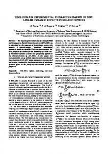
Simulation Tools The spreadsheet tools used in the simulation are graphics, formulas, macros, and toolbars. To simulate a basic block [5], the drawing toolbar is used to represent this block using, in some cases, its conventional drawing found in textbooks. Formulas are then used to calculate the block output as a function of the inputs and other parameters. These two steps are recorded in a macro whose code (in Visual Basic) is edited to ensure that all references are relative to the current active worksheet cell, which is considered the first input cell. The macro is next attached to a toolbar button. By clicking on this button, the macro will be executed, causing the block to be generated at the location of the active cell. To create an adder, for example, the drawing toolbar is used to draw the adder with three inputs (C6, C7, and C8) and one output (E7) as shown in Fig. 1. The inputs are multiplied with scale factors stored at cells D6, D7, and D8 and initialized to one. These scaling factors can be directly modified on the worksheet by the user. The formula = C6*D6 + C7*D7 + C8*D8, which relates the output to the in-
El-Hajj (
[email protected]), Kabalan, and Khoury are with the American University of Beirut, Faculty of Engineering and Architecture, Electrical and Computer Engineering Department, P.O. Box 11-0236, Beirut, Lebanon. 0272-1708/00/$10.00©2000IEEE 8
IEEE Control Systems Magazine
December 2000
put, is written at cell E7. This process of drawing and writing formulas is recorded in a macro called “Adder” and linked to a button called “Adder” that is included in a toolbar called “linear control toolbox.” This toolbar is constructed to graphically simulate any linear control system. As shown in Fig. 1, to generate the second adder, cell H9 is made the active cell and the Adder button is clicked. To manage the simulation process, a resetting and a running mechanism is implemented. This is done using some variables stored in the upper rows of the worksheet. An initialization flag stored in cell B1 is set to zero when no calculation is required and is set to one when a calculation is requested. Some blocks use this flag to reset their states to preset initial conditions. A counter is stored in cell B2 to indicate the number of iterations (i.e., spreadsheet calculations) that are performed. This counter is initialized to zero and incremented for each worksheet calculation. This is done by writing at cell B2 the formula = IF ($B$1 = 0;0;B2 + 1). The integration step is stored in cell B3, and the time is calculated and stored in cell B4 using the formula =$B$2 *$B$3. A spinner is used in cells F1-F2 to set the number of worksheet calculations to be performed in a single run. The resetting mechanism is created using the Reset button. The underlying macro resets the initialization flag and the counter to zero. Resetting is needed before any new run, and the running mechanism is created using the Run button. The underlying macro sets the initialization flag to one and recalculates the worksheet the number of times indicated by the spinner. The “Run” macro can be executed many consecutive times using different spinner values. The simulation requires connecting an output cell of one block (source) to an input cell of another block (destination). This is done in two steps by drawing a line that connects the centers of the two cells and by writing in the destination cell a formula equal to the source cell address. In the first step, the source cell is made active and the Source button is clicked. The underlying macro calculates and saves the address of the source cell. In the second step, the destination cell is made active and the Destination button is clicked. The underlying macro calculates the
address of the destination cell, writes in this cell a formula equal to the source cell address, and draws a line that connects the centers of the source and destination cells. The Destination button will be active if clicked directly after the Source button. As an example, to connect the first adder output to the second adder input, as shown in Fig. 1, cell E7 is made the active cell, the Source button is clicked, then cell H9 is made the active cell, and the Destination button is clicked.
Integrator and First-Order System Simulations A first-order system is defined in the s domain by the transfer function Y ( s) 1 . = X( s) s + a
(1)
An integrator has the same transfer function as in (1) with a =0. The output y(t ) is obtained as a function of the input x(t ) by solving dy = f ( x, y ) = −ay + x dt
(2)
with y(0) = y0 = 0. Equation (2) can be written in discrete form using the integration step h as follows: yi + 1 = yi + f ( xi , yi )h = yi + ( −ayi + xi )h. Many methods discussed in [7] can be used to calculate the output sequence yi given an input sequence xi . An approach similar to the Heun method is used in this simulation, but other methods can be used as well when more or less accuracy is needed. In this method, the value of yi +1 is predicted using the predictor equation yi0+ 1 = yi + f ( xi , yi )h.
(3)
An improved value of yi +1 is next obtained using the corrector equation
yi + 1 = yi +
f ( xi , yi ) + f (xi + 1 , yi0+ 1 ) 2
h. (4)
In the case of the first-order system (1), the predictor and corrector equations become
Predictor: yi0+ 1 = yi + ( −ayi + xi )h, Figure 1. Simulation tools.
December 2000
(5)
IEEE Control Systems Magazine
9
Corrector: yi + 1 = yi +
(−ay + x − ay i
0 i +1
i
+ xi + 1 )
2
h.
(6)
In the case of an integrator, a =0 and the two previous equations are reduced to the trapezoidal rule [7] yi + 1 = yi +
( xi + xi + 1 ) h. 2
the case a =0 gave the same results as the integrator. This simulation was also tested on more complicated examples as discussed in the “Illustrative Examples” section.
Second-Order System Simulation In this section, we define the simulation of the second-order system. This system is defined in the s domain by the transfer function
(7)
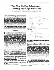
To simulate an integrator with input D6 and output F6, the drawing toolbar is used as shown in Fig. 2. For the correct operation of the integrator, xi and yi must be stored in two cells used to calculate the output yi +1 and then updated to new values used in the next iteration. Due to the row-wise calculation of the Excel worksheet, xi and yi are stored in cells calculated after F6 (for example, cells D7 and E7). The previous input value xi is stored in cell D7 by writing the formula = IF($B$1 = 0;0;D6) in this cell. The previous output value yi is stored in cell E7 by writing = IF($B$1 = 0;0;F6) in this cell . The output yi +1 is obtained at cell F6 by implementing (7) as follows:
Y ( s) as + b as −1 + bs −2 . = −2 = 2 U ( s ) s + cs + d ds + cs −1 + 1
(8)
A function X ( s ) is defined as X( s) =
Y ( s) U ( s) . = as −1 + bs −2 ds −2 + cs −1 + 1
Defining the functions X1 = s −2 X and X2 = s −1 X , the following expressions are then obtained: Y ( s ) = aX2 + bX1 U ( s ) = dX1 + cX2 + X .
(9)
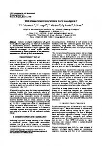
= IF($B$1 = 0;0;E7 + 0.5*$B$3*(D6 + D7)). As in the case of the adder, this process is automated using the Integrator toolbar button that is attached to the “Integrator” macro that draws and writes the integrator formulas using the active cell as the input cell of the integrator. Consider the simulation of a first-order system with the transfer function given in (1) using cell D6 as input and cell F6 as output. The drawing toolbar is used to draw it as shown in Fig. 3. The parameter a is stored in cell E5, initialized to zero, and can be changed at any time by the user. As in the case of the integrator, the previous input value xi is stored in cell D7 by writing = IF($B$1 = 0;0;D6) in this cell. The previous output value yi is stored in cell E7 by writing the formula = IF($B$1 = 0;0;F6) in this cell. The predicted output value yi0+1 of (5) is stored at cell E6 using
Using the definitions of X1 , X2 and (9), X1 , X2 , and U will then satisfy the following equations: sX1 = X2 sX2 = X = −dX1 − cX2 + U .
Figure 2. Integrator simulation.
= E7 + $B$3*( −E5*E7 + D7). The corrected output yi +1 is obtained at cell F6 by implementing (6) as follows: = IF($B$1 = 0;0;E7 + 0.5*$B$3*( −E5*E7 + D7 − E5*E6 + D6)). As in the case of the adder and the integrator, the first-order system is customized using the First toolbar button. To test this simulation, many runs were considered. Examples with known analytical solutions were tried, and it was found that the simulation result matches the exact solution. On the other hand, the first-order system with
10
Figure 3. First-order system simulation.
IEEE Control Systems Magazine
December 2000
Figure 4. Second-order system simulation. (10) Assuming that x1 (0) = x 2 (0) = 0, (10) can be written in the time domain as dx1 = f1 ( x1 ,x 2 ,u ) = x 2 dt
(11)
Fig. 4 shows a second-order system block with transfer function given in (8) using cell D6 as input and cell G6 as output. The drawing toolbar is used to draw it, and the parameters a, b, c, and d are stored in cells E4, F4, E5, and F5, respectively. All these parameters are initialized to zero, but their values can be changed at any time by the user. In Fig. 4, the parameter values are:a =1, b = 2, c = 6, andd =5. As in the case of the integrator, the previous input value ui is stored in cell D7 by writing = IF($B$1 = 0;0;D6) in this cell. To implement (14)-(18), x10,i + 1 is stored in cell D5, x 20,i + 1 in cell G5, x1 ,i + 1 in cell E6, x 2 ,i + 1 in cell F6, x1,i in cell E7, and x 2,i in cell F7. x10,i + 1 is calculated by implementing formula (14) in cell D5 as follows: = E7 + $B$3*F7. x 20,i + 1 is calculated by implementing formula (15) in cell G5 as follows: = F7 + $B$3*( −F5*E7 − E5*F7 + D7).
dx 2 = f2 ( x1 ,x 2 ,u ) = −dx1 − cx 2 + u. dt
(12)
The output y(t ) is found to be y(t ) = ax 2 (t ) + bx1 (t ).
x1 ,i + 1 is calculated by implementing formula (16) in cell E6 as follows: = E7 + 0.5*$B$3*(F7 + G5).
(13)
Equations (11)-(13) can be written in discrete form using the integration step h. The same method used in the case of the first-order system is used to solve (11) and (12). The variables x1 and x 2 are predicted using an equation similar to (3):
x 2 ,i + 1 is calculated by implementing formula (17) in cell F6 as follows: = F7 + 0.5*$B$3*( −F5*E7 − E5*F7 + D7 − F5*D5 − E5*G5 + D6). x1,i is calculated by implementing in cell E7
x10,i + 1 = x1 ,i + x 2 ,i h,
(14)
x 20,i + 1 = x 2 ,i + ( −dx1 ,i − cx 2 ,i + ui )h.
(15)
= IF($B$1 = 0;0;E6). x 2,i is calculated by implementing in cell F7 the formula = IF($B$1 = 0;0;F6).
The corrected values x1 ,i + 1 and x 2 ,i + 1 are obtained using equations similar to (4): x1 ,i + 1 = x1 ,i +
x 2 ,i + 1 = x 2 ,i +
x 2 ,i + x 20,i + 1 2
(
The output yi +1 is finally obtained by implementing formula (18) in cell G6 as h,
(16)
( −dx1 ,i − cx 2 ,i + ui ) + −dx10,i + 1 − cx 20,i + 1 + ui +1 2
) h.
(17) The output yi +1 with the initial condition y(0) = y0 = 0 is then given by yi + 1 = ax 2 ,i + 1 + bx1 ,i + 1 .
December 2000
(18)
= E4*F6 + F4*E6. As in the case of the previous blocks, the second-order system is customized using the Second toolbar button and then tested.
Illustrative Examples To illustrate the method, two examples are considered, and the results are compared with the actual values. In the first example, a unity feedback linear control system, the plant
IEEE Control Systems Magazine
11
transfer function is a second-order system represented by the following transfer function [8, Ex. 10-3]: G( s ) =
4500K . s( s + 361.2)
This system is controlled by a proportional integral (PI) controller with gain K=181.2. The spreadsheet simulation of this linear system is shown in Fig. 5. In this simulation, the controller is represented by an integrator and an adder connected in a parallel/cascaded fashion. The parameters KI Figure 5. Spreadsheet simulation of example 1. and KP are stored in cells I2 and I3, respectively, and referenced at the adder’s inputs us- values are stored in range [B14-B114] by multiplying the ing formulas. A second-order block is used to simulate the counter values in range [A14-A114] by the step in cell B3. plant transfer function with appropriate coefficients. The Successive outputs at cell M6 (named OUTPUT) are stored output of the second-order block is used as input to the first in range [C14-C114] by writing in cell C14 the formula adder for the next iteration. Since Excel calculates its cells = IF($B$1 = 0;0;IF(A14 = $B$2;OUTPUT;C14)). by rows from left to right, the ordering and placement of devices should be done carefully and the output formulas of This formula is copied to the range [C15-C114]. The Excel some adders should be edited. In this example, the formula at the second adder’s output is edited to refer to cell F6 in- chart toolbar is then used for plotting the system responses stead of H7, since H7 represents the value of F6 at the previ- as shown in Fig 6. Good agreement with the results in [8] is ous iteration at the time when J6 is calculated. For the same obtained. As a second example, consider the compensated system reason, the input to the first adder at cell D7 is edited to refer directly to the system output =M6. An alternative would be shown in Fig. 7. A spreadsheet simulation of this system is to change the connection path (M6, M9, D9, D7) to another shown in Fig. 8. The simulation of the linear transfer function is path such as (M6, M3, D4, D6). In this last path, the input D6 done in the same way as in the previous example. The reis used instead of D7, and due to the calculation of the worksheet by rows, the present value of D6 is equal to the value of M6 at the previous worksheet calculation. In this case, it is not necessary to edit the content of D6 to refer directly to the content of M6. The unit step response is calculated by applying a unit step function at the input of the system, as indicated in cell D5. For comparison, the same values considered in [8] are also considered in this case; that is, KP = 0.08 and KI = 0.08, 0.8, and 1.6. The corresponding system responses are arranged in adjacent columns. To record the output values for counter values 0,5,10..., the range [A14-A114] is filled with multiples of five from 0 to 500. The corresponding time Figure 6. Unit step response of the system shown in Fig. 5.
12
IEEE Control Systems Magazine
December 2000
r(t )
K(s+2) ______ s+1
1 ___________ s2+2s+4
c(t )
Figure 7. Block diagram of example 2.
Figure 8. Spreadsheet simulation of the system shown in Fig. 7. sponse of the system is plotted in Fig. 9 by following an approach similar to that in the previous example. The results are in agreement with those obtained in [9] for the same example.
Discussion
The size of the worksheet containing the code and the toolbar is on the order of 75 kb. Thus only limited computer resources are needed to run the application. Furthermore, this method is easy to use and simply requires learning the function of each of the eight toolbar buttons. To analyze and plot the results, the spreadsheet data processing facilities can be used, which allows an iterative step-by-step or continuous run of the simulated system. This procedure shows the values at the output of any block in the worksheet. The outputs with different parameter value(s) can be simply obtained and plotted using the what-if feature of spreadsheets. This method is also sufficiently accurate for a large number of practical applications, since Excel stores numbers and performs calculations using 15 digits of precision. To increase the accuracy of the results, the integration step can be reduced or more sophisticated formulas can be used in simulating some blocks [7]. Reducing the integration step may lead to an increase in the number of iterations (worksheet calculations), however, which makes this method slow in simulating large control systems. In summary, this method is low in cost and suitable for quick simulation when the user lacks the time or means to write a sophisticated program or access a more sophisti-
The method presented has its advantages and limitations when compared with related simulation packages. As an example, MATLAB-Simulink is an advanced software package widely used by engineers, students, and instructors for simulating control systems. Several undergraduate and graduate students in our university have copies of the package and had to spend some time learning it. The main advantage of the current simulation method is its use of spreadsheets that are widely available on most computers (definitely more than MATLAB) and are familiar to a large class of users. Due to our familiarity with spreadsheets, it was possible to develop this application using macros and formulas. This approach considerably reduced the programming effort that is usually required to develop similar applications (see the “Simulation Tools” section). The code obtained (in Visual Basic) consists of a few pages that can be directly accessed by users. Figure 9. Unit step response of the system shown in Fig. 7.
December 2000
IEEE Control Systems Magazine
13
cated package (i.e., MATLAB). It is useful in educational settings where budgets and resources are sometimes limited, especially since a worksheet copy of this package can be obtained from the Web (http://www.aub.edu.lb/~elhajj) at no cost.
Conclusion A new method has been presented for simulating linear control systems using modern spreadsheet programs. The method is characterized by its flexibility, simplicity, and availability. It has been verified for various cases, and examples were given for illustration. It is particularly useful for educational exercises that require calculations to be repeated with different parameters and values.
Acknowledgment This work is supported by the American University of Beirut Research Board.
References [1] A. El-Hajj and K.Y. Kabalan, “A spreadsheet simulation of logic networks,” IEEE Trans. Educ., vol. 34, pp. 43-46, 1991. [2] A. El-Hajj, K.Y. Kabalan, and M. Yehia, “Simulation of a class of integrated circuits using spreadsheets,” Proc. Inst. Elect. Eng., vol. 139, pt. G, no. 5, pp. 607-610, 1992. [3] A. El-Hajj and K.Y. Kabalan, “Time domain analysis of linear control systems using spreadsheets,” IEEE Trans. Educ., vol. 38, no. 4, pp. 317-320, 1995. [4] K.Y. Kabalan, A. El-Hajj, and W. Smari, “Nonlinear and sampled data control systems analysis using spreadsheets,” Proc. Inst. Elect. Eng., vol. 143, pt. A, no. 1, pp. 52-56, 1996. [5] A. El-Hajj and M. Hazim, “On using spreadsheets for logic networks simulation,” IEEE Trans. Educ., vol. 41, no. 4, pp. 311-319, 1998. [6] A. El-Hajj, “Functional simulation using spreadsheets,” Simulation, vol. 73, no. 2, pp. 80-90, Aug. 1999. [7] S.C. Chapra and R.P. Canale, Numerical Methods for Engineers. New York: McGraw-Hill, 1990. [8] B.C. Kuo, Automatic Control Systems, 7th ed. Englewood Cliffs, NJ: Prentice Hall, 1995. [9] R.C. Dorf and R.H. Bishop, Modern Control Systems. Reading, MA: Addison Wesley, 1995.
14
Ali El-Hajj was born in Aramta, Lebanon. He received the B.S. degree in physics from the Lebanese University, Lebanon, in 1979; the degree of “Ingenieur” from L’Ecole Superieure d’Electricite, France, in 1981; and the “Docteur Ingenieur” degree from the University of Rennes I, France, in 1983. From 1983 to 1987, he was with the Electrical Engineering Department at the Lebanese University. In 1987, he joined the American University of Beirut where he is currently Professor of Electrical and Computer Engineering. His research interests are numerical solution of electromagnetic field problems and engineering education. Karim Y. Kabalan was born in Jbeil, Lebanon. He received the B.S. degree in physics from the Lebanese University in 1979 and the M.S. and Ph.D. degrees in electrical engineering from Syracuse University in 1983 and 1985, respectively. During the 1986 fall semester, he was a visiting Assistant Professor of Electrical Engineering at Syracuse University. Currently, he is a Professor of Electrical Engineering with the Electrical and Computer Engineering Department, Faculty of Engineering and Architecture, American University of Beirut. His research interests are numerical solution of electromagnetic field problems and software development. Shahwan V. Khoury was born in Lebanon. He received his B.E. degree in electrical engineering from Youngstown State University in 1960 and his M.S. and Ph.D. degrees from Carnegie Mellon University in 1961 and 1964, respectively. He was a member of the Technical Staff (AT&T), Technical Director at Projects Studies and Implementation, San Francisco; Manager of Electromechanical Contracts with Kettaneh, Lebanon; General Manager, Debbas Enterprise, Lebanon; and Consultant, SDI, London. Currently, he is an Associate Professor of Electrical and Computer Engineering at the American University of Beirut. His research interests are in numerical solution of electromagnetic field problems and software development.
IEEE Control Systems Magazine
December 2000