ItCompress: An Iterative Semantic Compression Algorithm H. V. Jagadish1
Raymond T. Ng2
Beng Chin Ooi3
Anthony K. H. Tung3
+
1
University of Michigan. email:
[email protected] 1301 Beal Ave, Ann Arbor, MI, 48109-2122 University of British Columbia. email:
[email protected] 2366 Main Mall, Vancouver, B.C., V6T 1Z4 National University of Singapore, email:{ooibc, atung}@comp.nus.edu.sg 3 Science Dr 2, Singapore 117543 4 +Contact Author 2
3
Abstract
2. Data values essential for deriving the data values in (1) using M .
Real datasets are often large enough to necessitate data compression. Traditional ‘syntactic’ data compression 3. Data values that do not fit M i.e., outliers. methods treat the table as a large byte string and operate at By storing only the model M together with the second the byte level. The tradeoff in such cases is usually between and third groups of data values, compression is achieved the ease of retrieval (the ease with which one can retrieve since M typically takes up substantially less storage space a single tuple or attribute value without decompressing a than the original database. Such semantic compression genmuch larger unit) and the effectiveness of the compression. erally has the following advantages over syntactic compresIn this regard, the use of semantic compression has gension: erated considerable interest and motivated certain recent works. • More Complex Analysis In this paper, we propose a semantic compression alSince the semantics of the data are taken into consideragorithm called ItCompress ITerative Compression, which tion, complex correlation and data dependency between achieves good compression while permitting access even the data attributes can be exploited in case of semantic at attribute level without requiring the decompression of compression of data. Note that this is not supported in a larger unit. ItCompress iteratively improves the comcase of syntactic compression methods since the database pression ratio of the compressed output during each scan is viewed as a large byte string in such methods. Furof the table. The amount of compression can be tuned ther, the exploratory nature of many data analysis applibased on the number of iterations. Moreover, the initial cations implies that exact answers are usually not needed iterations provide significant compression, thereby making and analysts may prefer a fast approximate answer with it a cost-effective compression technique. Extensive exan upper bound on the error of approximation. By taking periments were conducted and the results indicate the suinto consideration the error tolerance that is acceptable periority of ItCompress with respect to previously known in each attribute, semantic compression can be used to tehniques, such as ‘SPARTAN’ and ‘fascicles’. perform lossy compression to enhance the compression ratio. (The benefits can be substantial even when the level of error tolerance is low).
1
Introduction
Advances in information technology have necessitated the creation of massive high-dimensional tables required for new applications such as corporate data warehouses, network-traffic monitoring and bio-informatics. The sizes of such tables are often in the range of terabytes, thereby making it a challenge to store them efficiently. In order to reduce the respective sizes of such tables, an obvious solution is the use of traditional data compression methods which are statistical or dictionary-based (e.g., Lempel-Ziv [17]). Such methods are ‘syntactic’ in nature since they view the table as a large byte string and operate at the byte level. More recently, compression techniques, which take semantics of the table into consideration during compression [9, 1], have received considerable attention. In general, these algorithms first try to derive a descriptive model, M , of the database by taking into account the semantics of the attributes and then separate them into the following three groups with respect to M : 1. Data values that can be derived from M .
• Fast Retrieval Given a massive table, only certain rows of the table are typically accessed to answer database queries. As such, it is desirable to be able to decompress only certain tuples in the database, while allowing the other tuples to remain uncompressed. Since syntactic compression methods, such as gzip, are unaware of the record boundary, it is usually not possible to do so without uncompressing the whole database. In fact, it has even been suggested [12, 13] that tables are better compressed column-wise. Separate compression of individual tuples, and even individual attributes, is possible. However, syntactic compression is usually not effective on very small strings. As such, this sort of fine granularity compression is not used frequently. Semantic compression permits local reconstruction of selected tuples and even attributes without having to reconstruct the entire table. In fact, it is even possible to store the compressed data in a relational database, thereby making the query optimization and indexing techniques of relational databases available also for compressed data.
• Query Enhancement In addition to the compression itself, there could be intrinsic value in obtaining the descriptive model M for semantic compression. For example, in [1] where M is a set of classification or regression trees, the following rule could have been found “if X = a, then Y = b with 100% accuracy”. In such a case, for a query searching for tuples with X = a and Y = c, an empty answer set could be returned very efficiently. Such side benefits are not available when syntactic compression is used.
age 20 25 30 40 50 60 70 75
salary 30,000 76,000 90,000 100,000 110,000 50,000 35,000 15,000
assets 25,000 75,000 200,000 175,000 250,000 150,000 125,000 100,000
credit poor good good poor good good poor poor
sex male female female male female male female male
(a) An Example Table
Although semantic compression has several advantages over syntactic compression, the two types of compression are not mutually exclusive. In fact, it has been shown in [9] that applying semantic compression before syntactic compression results in better compression performance than from either syntactic compression or semantic compression. (However, syntactic compression used in the second phase will nullify the fast retrieval benefit discussed earlier for semantic compression.) In this paper, we propose a new semantic compression scheme based on the selection of representative rows. Each tuple in the table is assigned to one of the representative rows and its attribute values are defaulted to be the same with the assigned representative rows unless the actual value differs from the default value by more than an acceptable error threshold. In such cases, outlying values are specifically stored for the row. Our scheme is similar to clustering, with each representative row considered like a cluster representative. However, there is a significant difference due to the outlying values that are possible. These attributes could have values in a row wildly different from its assigned representative row. As such, by most standard metrics, the distance between a row and its representative could be very large. Let us illustrate the concept with an example:
RRid 2 1 1 1 1 1 2 2
Bitmap 01011 11011 11111 01100 01111 01110 11110 11111
Outlying Values 20, 25,000 75,000 40, poor, male 50 60, male female
(b) Table Tc
RRid 1 2
age 30 70
salary 90,000 35,000
assets 200,000 100,000
credit good poor
sex female male
(c) Representative Rows
Figure 1. Representative Rows and Compressed Table tive rows may keep changing, each iteration monotonically improves the global quality. In fact, for many cases, the rate of convergence is high i.e., even a small number of iterations may be sufficient to deliver significant compression performance. Furthermore, each iteration of the algorithm requires only a single scan over the data, leading to a fast compression scheme. The rest of this paper is organized as follows. Section 2 gives a formal definition of the problem of semantic data compression, while our proposed ItCompress algorithm is presented in Section 3. In Section 4, we briefly describe competing approaches, and discuss their comparative merits. In Section 5, we present results from an extensive experimental study comparing our approach with these approaches. Section 6 describes other related work, while Section 7 concludes with directions for future work.
Example 1 Consider the table in Figure 1(a) which contains 5 attributes and 8 tuples. Let the acceptable error threshold for the numeric attributes age, salary and assets be 5, 25,000 and 50,000 respectively, while no errors are allowed for categorical data. We show a selection of representative rows in Figure 1(c) and the compressed table in Figure 1(b). As can be seen, each row in the compressed table is associated with one of the representative rows using a representative row ID (RRid). A bitmap is assigned to each row to provide the position for the outlying values. A ‘1’ at the nth bit indicates that its nth attribute value is within an acceptable error tolerance threshold of the nth attribute value for the representative row, while a ‘0’ indicates otherwise. Thus from the bitmap in the first row, we can see that the values for attribute “age” and “assests” in that row are ‘20’ and ‘25,000’ respectively instead of ‘30’ and ‘200,000’ as indicated by its representative row. 2
2
Problem Description
Given a table T , which has m attributes X1 , ..., Xm and n rows, we use R[Xi ] to represent the value of Ai for row R. We denote the domain of attribute Xi as dom(Xi ). Our aim is to perform a lossy compression on T such that the values reconstructed from the compressed table satisfy certain error tolerances for each column. We denote these error tolerances as a vector e = [e1 , ..., em ] with ei being the error tolerance for Xi . The value ei is interpreted differently depending on the (domain) type of Xi . Our techniques are applicable irrespective of the specific definitions chosen for tolerance. For instance, we could use edit dis-
To compress data according to the scheme, the difficult issue is to choose a good set of representative rows. For this purpose, we develop an algorithm called ItCompress (ITerative Compression) which iteratively improves the set of chosen representative rows. From one iteration to the next, new representative rows may be selected, and old ones discarded. A key analytical result of this paper is the “convergence” theorem showing that, even though the representa2
Notation e ei f v(Xj , G(Pi ))
tances for string types, or distance to the closest common ancestor for classification types. To keep matters concrete, in all examples and experiments in this paper, we focus on two of the most popular types: An attribute Xi is said to be numeric if the values in dom(Xi ) can be ordered while attributes with unordered, discrete domain values are said to be categorical. With these, we associate the following tolerance rules:
G(Pi ) m n P Pi Pi [Xj ]
1. Categorical For a categorical attribute, the tolerance ei defines an upper bound on the probability that the approximate value of Xi in Tc is different from the actual value in T. This means that given Xi = x for a particular row in T and Xi = x0 for the same row in Tc , P rob(x = x0 ) ≥ 1 − ei .
Pmax (R) R R[Xj ] RRid T Tc X
2. Numeric Given that the value of an attribute Xi is x in T and that x0 is it corresponding value in Tc , then the tolerance ei defines the upper bound that x0 can deviate from x. This means that x should be within the range [x0 − ei , x0 + ei ].
Description error tolerance vector error tolerance for attribute Xi the most frequent value/interval for attribute Xi in group G(Pi ) a set of rows which have Pi as the best match number of attributes in a table number of rows in a table a set of representative rows the ith representative row in P value of attribute Xi for representative row Pi the representative row that best matches row R a row in a table T value of attribute Xi for row R representative row id a table a compressed version of T a set of attributes
Figure 2. Notations
Given the error tolerance specifications, our aim is to derive a compression scheme that minimizes total storage while satisfying these criteria.
Definition 2.2 Coverage Let R be a row in T and let Pi be a representative row in P . We say that the coverage of Pi on R, cov(Pi , R) is the number of attributes Xi in which R[Xi ] is matched by P [Xi ]. 2
Definition 2.1 Compression Scheme Given the table T , our basic compression scheme consists of two parts, the set of representative rows P and the compressed table Tc
As an example, the coverage of representative row P1 on the second row of T in Example 1 is 4 since the age, salary, credit, and sex attributes lie within the error tolerance. Now let us define the total coverage of a set of representative rows P on a table T .
1. Representative Rows The set of representative rows P consists of a set of k rows {P1 , ..., Pk } where each row Pi ∈ (dom(X1 )) × (dom(X2 )) × ...(dom(Xm )). We say that a row in R matches a representative row Pi on attribute Xi if one of the following conditions is true:
Definition 2.3 Total Coverage Let P be a set of representative rows P1 , ..., Pk and let the table T contain n rows R1 , ..., Rn . For each row, Ri let Pmax (Ri ) be the representative row from P that gives the maximum coverage among Pi (i ≤ i ≤ k) to Ri . We define P the total coverage of P on T to be totalcov(P, T ) = 2 i=1..n cov(Pmax (Ri ), Ri )
(a) P [Xi ] − ei ≤ R[Xi ] < P [Xi ] + ei if Xi is numeric (b) R[Xi ] = P [Xi ] if Xi is categorical 2. Compressed Table For each row R in T , the compressed table Tc has a corresponding row which can be further split into the following three parts: (a) A representative row id, RRid, which indicates that R is most similar to representative row PRRid in the set of representative rows. (b) A bitmap which has a bit for every attribute. A bit representing Xi is set to 1 if PRRID [Xi ] matches RRRiD [Xi ] and 0 otherwise. (c) An outlying list which stores attribute values in R that cannot be inferred satisfactorily from the representative row id and bitmap.
Maximizing the total coverage is equivalent to minimizing the number of outlying values and thus we have the following problem definition: Definition 2.4 Maximum Coverage (MC) Problem Given a table T , an error tolerance vector e and a userspecified value k, find a set of k representative rows P which maximizes totalcov(P, T ). 2 For ease of reference, we show in Figure 2 the notations used in this paper.
Given our compression scheme, one obvious conclusion is that if we can find a set of k representative rows, P = {P1 , ..., Pk } such that all rows are fully matched by at least one member from P , then the number of outlying values that need to be stored will be zero giving rise to very good compression ratio. However, this is not always possible and hence our aim is to minimize the number of outlying values that need to be stored using the notion of coverage.
3
The ItCompress Algorithm
The MC problem is easily shown to be NP-hard since a special case is equivalent to the k-center problem [5]. As such, our solution to this problem is to find an efficient 3
Algorithm ItCompress Input: A table T , a user specified value k and an error tolerance vector e. Output: A compressed table Tc and a set of representative rows P = {P1 , ..., Pk }. 1. 2. 3. 4. 5. 6. 7. 8.
RRid 1 2
age 20 25
salary 30,000 76,000
assets 25,000 75,000
credit poor good
sex male female
(a) Representative Rows
Pick a random set of representative rows P While totalcov(P, T ) is increasing do { For each row R in T , find Pmax (R) Recompute each Pi in P as follow: { For each attribute Xj , Pi [Xj ] = f v(Xj , G(Pi )) } }
age 20 60 70 75
salary 30,000 50,000 35,000 15,000
assets 25,000 150,000 125,000 100,000
credit poor good poor poor
sex male male female male
(b) G(P1 ):Rows assign to P1
age 25 30 40 50
Figure 3. The ItCompress Algorithm heuristic. While optimality is not guaranteed for our algorithm, experiments show that it gives a good compression ratio without sacrificing efficiency. The ItCompress (ITerative COMPRESSion) algorithm is presented in Figure 3. The algorithm begins by picking a random set of k representative rows from the table T . It then iteratively improves this random choice with the objective of increasing the total coverage over the table to be compressed. There are two phases in each iteration:
salary 76,000 90,000 100,000 110,000
assets 75,000 200,000 175,000 250,000
credit good good poor good
sex female female male female
(c) G(P2 ):Rows assign to P2
Figure 4. Iteration 1 for Example 2 row of the table are picked as the initial representative rows, we depict the situation for the first iteration of ItCompress in Figure 3. The representative rows P1 and P2 are shown in Figure 4(a) while Figure 4(b) and 4(c) show the rows that are assigned to P1 and P2 respectively. We leave it to readers to verify that each row is assigned to the representative row that best matches it (arbitrarily breaking ties). Having done so, P1 and P2 are recomputed by assigning to each attribute the most frequently occurring value/interval (highlighted in bold).
Phase 1: (Step 3 of ItCompress) In this phase, each row R in T is assigned to a representative row Pmax (R) that gives the most coverage to R among the members of P . Let G(Pi ) denote the set of rows that are assigned to a representative row Pi . Phase 2: (Steps 4 to 6 of ItCompress) In this phase, a new set of representative rows is computed. Each new Pi is computed by setting each attribute value Pi [Xj ] to be f v(Xj , G(Pi )) which denotes the most frequently occurring value/interval for attribute Xj in G(Pi ). For a categorical attribute, this can easily be done by keeping count of the number of occurrences for each categorical value in G(Pi ) during Phase 1. For a numeric attribute, f v(Xj , G(Pi )) is an interval of width [x − ej , x + ej ], x ∈ dom(Xj ) that is most frequently matched by the rows in G(Pi ). An efficient mechanism is to partition the range for Xj into micro-intervals of size that are significantly smaller than ej say ej /10 and keep track of the frequency of occurrence of each such micro-interval in Phase 1. A sliding window of size 2 ∗ ej is then moved along these sorted micro-intervals to find the range that is most frequently matched. This method ensures a linear time algorithm for computing f v(Xj , G(Pi )) while ensuring that the error in estimating f v(Xj , G(Pi )) is not more than the size of the micro-interval. The above two phases are repeated until there is no improvement in totalcov(P, T ). In some practical situations, it can also be specified that termination will occur if the improvement in totalcov(P, T ) is negligible in comparison to the previous iteration. Example 2 demonstrates the running of the ItCompress algorithm.
This new set of representative rows is shown in Figure 5(a) and we highlight the changes from the previous set of representative rows in bold. With this change, the rows in the table are again reassigned and only one of the row changes membership from G(P2 ) to G(P1 ). Note that the total coverage of the two representative rows improves from 25 to 31 as we move through the two iterations. The iterative process continues until there is no improvement in totalcov(P, T ). 2
Note that throughout the ItCompress algorithm, the error bound for categorical attribute is not utilized as part of the optimization. However, this can be easily done at the end of the algorithm. Given G(Pi ), the set of rows which have Pi as the best match, we can compute for each categorical attribute Xj , the frequency of occurrence of Pi [Xj ] within G(Pi ). Let us denote this frequency of occurrence as f req(Pi [Xj ], G(Pi )). Since we have an error tolerance of ej for Xj , we will remove up to ej /(1 − ej ) × f req(Pi [Xj ], G(Pi )) outlying values from the rows in G(Pi ) as long as these outlying values are in the domain of Xj . These removed outlying values can be assumed to be Pi [Xj ] without invalidating the error-bound. From here, we can see that ItCompress is indirectly utilizing the error tolerance for categorical attributes by trying to maximize coverage and thus allowing more outlying values to be removed.
Example 2 Consider again the table in Figure 1 and let us assume that the error tolerance vector e is {5, 25000, 50000, 0, 0 }. Assuming that k = 2 and that the first and second 4
RRid 1 2
age 70 25
salary 30,000 90,000
assets 125,000 175,000
credit poor good
each attribute. Assuming that the total number of domain values/intervals is d, then Phase 2 will have a run time complexity of O(kdl). Thus, the total run time complexity of ItCompress is O(kmnl + kdl). Since k, d, m and l are usually much less than n, we infer that ItCompress has a linear running time of O(n). To further reduce the running time in practice, we run ItCompress on a sample drawn from a large table and find a set of representative rows P for the sample. The remaining remaining rows in the table are then assigned to the best matched member in P . Experiments in the next section will show that a 5% to 10% sample is sufficient to produce good compression in this manner.
sex male female
(a) Representative Rows
age 20 40 60 70 75
salary 30,000 100,000 50,000 35,000 15,000
assets 25,000 175,000 150,000 125,000 100,000
credit poor poor good poor poor
sex male male male female male
(b) G(P1 ):Rows assign to P1
age 25 30 50
salary 76,000 90,000 110,000
assets 75,000 200,000 250,000
credit good good good
sex female female female
4
Two semantic compression algorithms [9, 1] have previously been suggested in the literature. Both these algorithms are quite complex, and the ItCompress algorithm described above appears to be much less sophisicated. While an extensive performance comparison will be presented in the next section, here we will highlight some of the differences and motivate some of the design choices made in ItCompress.
(c) G(P2 ):Rows assign to P2
Figure 5. Iteration 2 for Example 2
3.1
Discussion
Convergence and Complexity
Given the ItCompress algorithm described above, we have the following theorem:
4.1
Theorem 3.1 The total coverage of P on T is nondecreasing for every iteration in ItCompress.
Previously Known Semantic Compression Algorithms
In this section, we present a brief sketch of the two previously known semantic compression algorithms that we must compare ourselves against. The fascicles algorithm presented in [9] is the first semantic compression algorithm developed for tables and relations. Given a table of m columns and a user-specified value of u (u ≤ m), the algorithm extracts a model M consisting of w fascicles, each of which is represented by a u-tuple. The u columns are called compact attributes because these are columns with very similar values (i.e., values within the error tolerance) for all the rows assigned to the fascicle. While the fascicles algorithm determines the u compact columns locally on a per fascicle basis, SPARTAN [1] tries to separate the m columns into a set of predictor attributes and a set of predicted attributes globally for the entire relation. The model M , in this case, is simply the set of the predictor attributes. SPARTAN identifies the predictor columns by constructing Bayesian Network and CaRTs (classification and regression trees). As seen in the fascicle algorithm and SPARTAN, the key aspects that differentiate one semantic compression algorithm from another are the exact definition of the model M used to compress the database and how it is constructed.
Proof: Our aim is to show that the totalcov(P, T ) either increases or remain the same in both Phases 1 and 2. In Phase 1, this is trivial since each row is assigned a representative row Pi that provide the most coverage. If Pmax (Ri ) changed for a row Ri , then it means that cov(Ri , Pmax (Ri )) has increased, otherwise without a change in Pmax (Ri ),cov(Ri , Pmax (Ri )) would have remained the same. Since all rows either have the same or increased coverage for the same set of P , totalcov(P, T ) must have increased or remained the Psame. In Phase 2, we first observe that R∈G(Pi ) cov(R, Pi ) is equal P to j=1..m match(G(Pi ), Xj ) where match(G(Pi ), Xj ) is the number of rows in G(Pi ) that match Pi on attribute Xj . Since f v(Xj , G(Pi )) is chosen such that the number of rows from G(PP i ) that match Pi [Xj ] is maximum, we are also maximizing R∈G(Pi ) cov(R, Pi ). Since this is done for each pattern Pi ∈ P , we are thus increasing or maintaining totalcov(P, T ). As can be seen, both Phase 1 and 2 either increase or maintain totalcov(P, T ), thus proving the theorem. 2 From Theorem 3.1, we can conclude that ItCompress will eventually converge since totalcov(P, T ) is finite. We now look at the issue of efficiency. Since ItCompress iteratively goes through the n rows in the table and matches each of them against the k representative rows, the number of rows compared is kn. Each row comparison requires 2m operations, where m is the number of columns. Thus, the run-time complexity for Phase 1 is O(kmnl), where l is the number of iterations. In Phase 2, computing each new Pi requires going through all the domain values/intervals of
4.2
Simplicity and Directness
In both fascicles and SPARTAN, the process of compression can generally be separated into 2 steps. Step 1: Finding a set of patterns or rules. Step 2: Using the discovered patterns/rules in Step 1, form 5
the global model, M for compressing the database.
on feasible solutions by virtue of the choice of solution technique. SPARTAN imposes a constraint that each attribute must be either a predicted or predictor attribute globally. In consequence, SPARTAN is not able to exploit situations where there is only local “column-wise” dependency in a dataset (i.e., exhibited by a subset of the rows). For example, “age