Mar 11, 2015 - minimum sum-rate strategy in cooperative data exchange (CDE) systems. ... that achieves universal recovery (the situation when all the clients.
1
Iterative Merging Algorithm for Cooperative Data Exchange
arXiv:1503.03165v1 [cs.DS] 11 Mar 2015
∗ Research
Ni Ding∗ , Rodney A. Kennedy∗ and Parastoo Sadeghi∗ School of Engineering, College of Engineering and Computer Science, the Australian National University (ANU), Canberra, ACT 2601 Email: {ni.ding, rodney.kennedy, parastoo.sadeghi}@anu.edu.au
Abstract—This paper considers the problem of finding the minimum sum-rate strategy in cooperative data exchange (CDE) systems. In a CDE system, there are a number of geographically close cooperative clients who send packets to help the others recover a packet set. A minimum sum-rate strategy is the strategy that achieves universal recovery (the situation when all the clients recover the whole packet set) with the the minimal sum-rate (the total number of transmissions). We propose an iterative merging (IM) algorithm that recursively merges client sets based on an estimate of the minimum sum-rate and achieves local recovery until the universal recovery is achieved. We prove that the minimum sum-rate and a corresponding strategy can be found by starting the IM algorithm with an initial lower estimate of the minimum sum-rate. We run an experiment to show that the complexity of the IM algorithm is lower than the complexity of existing deterministic algorithms.
I. INTRODUCTION Due to the growing amount of data exchange over wireless networks and increasing number of mobile clients, the basestation-to-peer (B2P) links are severely overloaded. It is called the ‘last mile’ bottleneck problem in wireless transmissions. Cooperative peer-to-peer (P2P) communications is proposed for solving this problem. The idea is to allow mobile clients to exchange information with each other through P2P links instead of solely relying on the B2P transmissions. If the clients are geographically close to each other, the P2P transmissions could be more reliable and faster than B2P ones. Consider the situation when a base station wants to deliver a set of packets to a group of clients. Due to the fading effects of wireless channels, after broadcast via B2P links, there may still exist some clients that do not obtain all the packets. However, the clients’ knowledge of the packet set may be complementary to each other. Therefore, instead of relying on retransmissions from the base station, the clients can broadcast linear packet combinations of the packets they know via P2P links so as to help the others recover the missing packets. We call this kind of transmission method cooperative data exchange (CDE) and the corresponding system CDE system. Let the universal recovery be the situation that all clients obtain the entire packet set and the sum-rate be the total number of linear combinations sent by all clients. In CDE systems, the most commonly addressed problem is to find the minimum-sum rate strategy, the transmission scheme that achieves universal recovery and has the minimum sum-rate. This problem was introduced in [1]. Randomized and deterministic algorithms for solving this problem have been
proposed in [2], [3] and [4], [5], respectively. The idea of the randomized algorithms in [2], [3] is to choose a client with the maximal or non-minimal rank of the received encoding vectors and let him/her transmit once by using random coefficients from a large Galois field. But, these randomized algorithms repetitively call the rank function, the complexity of which grows with both the number of clients and the number of packets. On the other hand, the authors in [4], [5] propose deterministic algorithms where the complexity only grows with the number of clients. However, there are two problems with the deterministic algorithms in [4], [5]. One is that they both rely on the submodular function minimization (SFM) algorithm, and the complexity of SFM algorithms is not low.1 The other is that the algorithms in [4], [5] cannot be implemented in a de-centralized manner. In this paper, we propose an iterative merging (IM) algorithm, a deterministic algorithm, for finding the minimum sum-rate strategy in CDE systems. The IM algorithm starts with an initial estimate of the minimum sum-rate. It recursively merges the clients that require the least number of transmissions for both the local recovery and the recovery of the collectively missing packets. Here, local recovery means the merged clients exchange whatever missing in the packet set that they collectively know so that they share the same common knowledge and can be treated as a single entity. After the local recovery, the recovery of their collectively missing packets will be done by other clients. The IM algorithm iteratively achieves the local recovery in the merged clients until the universal recovery is finally reached. Also, the IM algorithm updates the estimate of minimum sum-rate whenever it finds that universal recovery is not achievable. We prove that the minimum sum-rate and a minimum sum-rate strategy can be found by starting the IM algorithm with a lower bound on the minimum sum-rate. By comparing the IM algorithm to the divide-and-conquer (DC) algorithm proposed in [4], we show that the IM algorithm is a bottom-up approach that can be implemented in a decentralized manner. We run an experiment to show that the complexity of the IM algorithm is O(K 3 · γ), where K is the number of clients and γ is the complexity of evaluating a submodular function. 1 There are many algorithms proposed for solving SFM problems. To our knowledge, the algorithm proposed in [7] has the lowest complexity O(K 5 · γ + K 6 ), where K is the number of clients, and γ is the complexity of evaluating a submodular function.
2
α∗S for the local recovery in S is determined by [4]3 client 2
client 4
{p1 , p4 , p7 , p8 }
{p1 , p2 , p6 }
client 1
client 3
{p3 , p4 , p6 , p7 , p8 }
{p3 , p4 , p5 , p6 , p7 , p8 }
Fig. 1. An example of CDE system: There are four clients that want to obtain eight packets. The has-sets are H1 = {p3 , p4 , p6 , p7 , p8 }, H2 = {p1 , p4 , p7 , p8 }, H3 = {p3 , p4 , p5 , p6 , p7 , p8 } and H4 = {p1 , p2 , p6 }.
α∗S = max
nl X |H | − |H | m S X : WS is a partition |WS | − 1 X ∈WS o of S that satisfies 2 ≤ |WS | ≤ |S| . (1)
Let WS∗ be the minimizer of (1). We call WS∗ the minimum sum-rate partition for local recovery in S, which imposes that a minimum sum-rate strategy must satisfy X rj = |HS | − |HS\X | (2) j∈X
WS∗
II. S YSTEM M ODEL AND P ROBLEM S TATEMENT Let P = {p1 , . . . , pL } be the packet set containing L linearly independent packets. Each packet pi belongs to the finite field Fq . The system contains K geographically close clients. Let K = {1, . . . , K} be the client set. Each client j ∈ K initially obtains Hj ⊂ P. Here, Hj is called the hasset of client j. The clients are assumed to collectively know the packet set, i.e., ∪j∈K Hj = P. The P2P wireless links between clients are error-free, i.e., information broadcast by any client can be heard losslessly by all other clients. The clients broadcast linear combinations of the packets in their has-sets in order to help each other recover P. For example, in the CDE system in Fig. 1, client 3 broadcasting p4 + p5 helps client 1 and client 2 recover p5 . Assume packet-splitting is not allowed. Let r = (r1 , . . . , rK ) be a transmission strategy with rj ∈ N0 being the total number P of linear combinations transmitted by client j. We call j∈K rj the sum-rate of strategy r. Let the universal recovery be the situation that all clients in K obtains the entire packet set P. The problem is to find a minimum sum-rate transmission strategy, a strategy that has the minimum sum-rate among all strategies that achieve universal recovery. III. I TERATIVE M ERGING A PPROACH In this section, we describe the idea of the IM scheduling method, present the algorithm and prove its optimality. We first clarify some notations and definitions as follows. Denote WK a partition of the client set K.2 Let |WK | be the cardinality of WK . We call WK a |WK |-partition of K. For example, WK = {{1, 2}, {3}, {4}} is a 3-partition of client set K = {1, 2, 3, 4}. Let Y ⊆ WK . We call Y the k-subset of partition WK if |Y| = k, e.g., {{2}, {3, 4}} is a 2-subset of partition WK = {{1}, {2}, {3, 4}}. Let Y˜ = ∪X ∈Y X , e.g., if Y = {{2}, {3, 4}}, Y˜ = {2, 3, 4}. For S ⊆ K such that |S| ≥ 2, denote HS = ∪j∈S Hj the set of collectively known packets in S. We define the local recovery in S as the situation such that all client j ∈ S obtains HS . For example, in Fig. 1, for S = {1, 3}, the problem of local recovery is how to let both client 1 and client 3 obtain the packet set H{1,3} = {p3 , · · · , p8 }. The minimum sum-rate 2 A partition W satisfies ∅ = 6 X ⊆ K, X ∩ X ′ = ∅ and ∪X ∈WK X = K K for all X , X ′ ∈ WK .
for all X ∈ [4]. It can be seen that the universal recovery is also the local recovery in S = K. The minimum sum-rate and minimum sum-rate partition for universal recovery are ∗ α∗K and WK , respectively. There exists a minimum sum-rate P ∗ . strategy satisfies j∈X rj = L − |HK\X | for all X ∈ WK ∗ Also, for all α ≥ αK , there exists a strategy that achieves the universal recovery and has the sum-rate equal to α. A. Iterative Merging Scheduling Method In this section, we propose a greedy scheduling method for the universal recovery in CDE systems, which is the basis for the IM algorithm we will describe in the next subsection.. We assume that the clients in CDE system can form coalitions, or groups. A coalition can contain just one client, and each client must appear in no more than one coalition. Any form of coalition in K can be represented by a partition WK , and any k-subset Y of WK contains k coalitions in WK . The idea of this scheduling method is to iteratively merge coalitions and achieve local recovery until the universal recovery is achieved. At the beginning, we assume that each client forms one coalition, which can be denoted by a Kpartition WK = {{j} : j ∈ K}. Let α be an estimate of α∗K . For example, α can be the lower bound on α∗K proposed in [2], [8] or the upper bound on α∗K proposed in [2]. We start an iterative procedure. In each iteration, we perform two steps: 1. Let k ∈ {2, · · · , |WK |}. We choose Y as a k-subset with the minimum value of k that satisfies the conditions X |HY˜ − HX | + L − |HY˜ | < α, (3) |Y| − 1 X ∈Y
X |HY˜ − HX | + L − |HY˜ | |Y| − 1
X ∈Y
≤
X |HY˜ ′ − HX | + L − |HY˜′ |, |Y ′ | − 1 ′
(4)
X ∈Y
for all other subsets Y ′ such that |Y| = |Y ′ |. Achieve local ˜ and update WK by merging all coalitions recovery in Y, X in Y into one coalition. 3 Eq. (1) was originally proposed in [9] for solving a secrecy generation problem. It is shown in [4] that Eq. (1) is also a method to determine the minimum sum-rate in CDE P systems. Eq. (1) is based on the condition for the local recovery [5]: j∈S\X rj ≥ |HS | − |HX | for all X ⊂ S, which means that the total amount of information sent by set S \ X must be complementary to that collectively missing in set X . Therefore, P P |HS |−|HX | ⌉ must be satisfied for all α∗S = j∈S rj ≥ ⌈ X ∈WS |WS |−1 partition WS .
3
P X| 2. If α < ⌈ X ∈WK L−|H |WK |−1 ⌉, terminate iteration, increase α by one and start the IM scheduling method (from Kpartition) again; Otherwise, go to step 1 until the universal recovery is achieved. In step 1, the interpretations of the conditions (3) and (4) are as follows. Based on Condition (4), Y must be the minimum sum-rate partition for the local recovery of the collectively |HY˜ −HX | ˜ i.e., Y = W ∗ .4 . So, P known packets in Y, ˜ X ∈Y |Y|−1 Y ˜ incurs the minimum sum-rate for the local recovery in Y. L − |HY˜ | is the number of collectively missing packets the recovery of which relies on the transmissions in client set ˜ If condition (3) is breached, it means that universal K \ Y. recovery with sum-rate α is not possible if the coalitions in Y ˜ Therefore, it is better for are merged to form one coalition Y. them to work individually than together. Condition (4) means that Y require less number of transmissions for the recovery of both collectively known and collectively missing packets than any other Y ′ such that |Y ′ | = |Y|. As discussed in Section III, if we find that condition l X L − |H | m X α≥ (5) |WK | − 1 X ∈WK
does not hold for some partition WK in step 2, it means α < α∗K and universal recovery is not possible with the sum-rate α. Therefore, α should be increased. Example 3.1: Consider applying the IM scheduling method in the CDE system in Fig. 1 with α = 6. The procedure is: • Assume that each client works individually at the beginning and initiate WK = {{1}, {2}, {3}, {4}}. It can be shown that coalitions {1} and {3} require 3 transmissions for local recovery and recovery of the collectively missing packet set {p1 , p2 }, which is less than any other two coalitions, i.e., 2-subset Y = {{1}, {3}} satisfies condition (4). Also, since 3 < α = 6, Y = {{1}, {3}} satisfies the condition (3). Therefore, coalitions {1} and {3} should be merged to form one coalition {1, 3} so that WK is updated as WK = {{1, 3}, {2}, {4}}. The problem of the local recovery in coalition {1, 3} is not difficult to solve. It is straightforward to see that {{1}, {3}} is the minimum sum-rate partition for ∗ local recovery in {1, 3}, i.e., W{1,3} = {{1}, {3}}. According to (2), r1 = |H{1,3} | − |H{3} | = 0 and r3 = |H{1,3} | − |H{1} | = 1. After local recovery, client 1 and client 3 have the same has-set. Therefore, the hasset of coalition {1, 3} is H{1,3} = {p3 , · · · , p8 }. At this moment, the transmission strategy is r = (0, 0, 1, 0). One can show that condition (5) holds for WK . So, we continue to the next iteration. • For WK = {{1, 3}, {2}, {4}}, one can show that Y = {{1, 3}, {2}} is a 2-subset that satisfies the conditions (3) and (4). So, coalitions {1, 3} and {2} is merged as {1, 2, 3}, and WK is updated as WK = {{1, 2, 3}, {4}}. One can show that {{1, 3}, {2}} is the minimum sumrate partition P for the local recovery in {1, 2, 3}, which imposes j∈{1,3} rj = |H{1,2,3} | − |H{2} | = 3 and 4 We
will show that this is the case in the proof of Theorem 3.4 in Section III-B
r2 = |H{1,2,3} | − |H{1,3} | = 1. By comparing to the current transmission strategy r = (0, 0, 1, 0), there should be 2 excessive transmissions from coalition {1, 3} and 1 excessive transmissions from coalition {2}. We can directly updated r2 to 1. Since clients 1 and 3 have the same has-sets, the excessive 2 transmissions can be completed by either client. We assume the client 1 does the excessive transmissions, i.e, r1 is updated to 2. We have transmission strategy r = (2, 1, 1, 0). Since condition (5) holds for WK , we continue to the next iteration. • For WK = {{1, 2, 3}, {4}}, we do not need to consider conditions (3) and (4) to merge the coalitions. The universal recovery can be achieved by the local recovery between coalitions {1, 2, 3} and {4}. One Pcan show that ∗ WK = {{1, 2, 3}, {4}}, which imposes j∈{1,2,3} rj = L−|H{4} | = 5 and r4 = L−|H{1,2,3} | = 1. We let client 2 to complete the 1 excessive transmission in coalition {1, 2, 3} and set r4 = 1. The transmission strategy is updated as r = (2, 2, 1, 1). It can be shown (by other method) that the minimum sum-rate is α∗K = 6 and (2, 2, 1, 1) is one of the minimum sum-rate strategies. Example 3.2: Consider applying the IM scheduling method in the CDE system in Fig. 1 with α = 5. It can be show that WK is updated as WK = {{1, 3}, {2}, {4}} in the P X| first iteration. But, since ⌈ X ∈WK L−|H |WK |−1 ⌉ = 6 > 5, condition (5) is breached. The iteration terminates, and α is updated as α = 6. We initiate WK = {{1}, {3}, {2}, {4}} and start the IM scheduling method again, where the same procedure as in Example 3.1 is repeated. Example 3.3: If the IM scheduling method is applied to the CDE system in Fig. 1 with α = 7. One can show that the same procedure as in Example 3.1 is repeated since condition (5) satisfied at each iteration. At the end, we have the transmission strategy r = (2, 2, 1, 1). But, α = 7 imposes a sum-rate equals 7. Since the universal has been achieved already, the excessive 1 transmission can be added to any client j ∈ K. For example, the strategy can be updated as r = (2, 2, 2, 1). B. Iterative Merging Algorithm We describe the IM scheduling method as the IM algorithm in Algorithms 1, 2 and 3. In Algorithm 1, vα is defined as vα (X ) = α − L + |HX |,
(6)
P
and α > X ∈WK vα (X ) is equivalent to the breach of condition (5). In Algorithm 2, X ˜ − ξα (Y) = vα (Y) vα (X ). (7) X ∈Y
′
ξα (Y) < 0 and ξα (Y) ≤ ξα (Y ) are equivalent to conditions (3) and (4), respectively. The set U returned by Algorithm 2 contains k-subsets such that the coalitions in each ksubset should be merged. For example, for the CDE system in Fig. 1, when WK = {{1}, {2}, {3}, {4}} and α = 6, FindMergeCand(WK , α) returns U = {{{1}, {3}}}.5 So, {1} 5 In this case, U contains one 2-subset of W . It is possible that U contains K several k-subsets. For example, if U = {{{1}, {3}}, {{2}, {4}}}, coalitions {1} and {3} merges, and coalitions {2} and {4} merges.
4
Algorithm 1: Iterative Merge (IM)
Algorithm 3: UpdateRates (update rates) input : merge candidate set U, transmission strategy r, sum-rate α output: updated transmission strategy r
input : sum-rate α output: sum-rate α, transmission strategy r 1 2 3 4 5 6 7 8 9 10 11 12 13 14 15
Initiate a K-partition WK = {{j} : j ∈ K} and a K-dimension transmission strategy r = (0, · · · , 0); repeat U = FindMergeCand(WK , α); r = UpdateRates(r, U); forall the Y ∈ U do update WK by merging all X ∈ Y; end P until |W PK | = 2, U = ∅ or α > X ∈WK vα (X ); if α > X ∈WK vα (X ) then α = α + 1; go to step 1; else r = UpdateRates(r, P {WK }); rj ′ = rj ′ + α − j∈K rj , where j ′ is the client that is randomly chosen in set K; endif
Algorithm 2: FindMergeCand (find merging candidate) input : a partition of client set WK , sum-rate α output: U, the set contains all candidates for merge 1 2 3 4 5 6
7 8 9 10
k = 1; repeat k = k + 1; U = ∅; forall the Y that is a k-subset of WK do if ξα (Y) < 0 and ξα (Y) ≤ ξα (Y ′ ) for all other k-subsets Y ′ such that Y ∩ Y ′ 6= ∅, Y ∩ Z = ∅ for all Z such that Z ∈ U then U = U ∪ Y; endif end until k = |WK | − 1 or U = 6 ∅;
and {3} merges. In Algorithm 3, ∆r calculates excessive number of transmissions (as described in Example 3.1). Theorem 3.4: The IM algorithm returns α∗K if α < α∗K and α if α ≥ α∗K . Proof: Consider the Queyranne’s algorithm [10] M := M ∪ {e} where e = arg min{vα (M ∪ {e}) − vα ({e}) : e ∈ K \ M}. Let WK be a partition generated by the IM algorithm. For any X ∈ WK such that X is not a singleton, if we start the Queyranne’s algorithm with M(0) = S ⊂ X , we will get M(|X |−|S|) = X .6 Due to the crossing submodularity of vα [5], at any iteration m ∈ {2, · · · , K − 1} of Queyranne’s algorithm [10] vα (M(m) ) + vα ({j}) ≤ vα (M(m) \ S) + vα (S ∪ {j}), (8) for all j ∈ K \ M(m) and S such that ∅ 6= S ⊆ M(m−1) .7 Also, the clients in P Y merges only if ξα (Y) < 0. WK satisfies P ′ v (X ) ≤ α X ∈WK X ∈W ′ vα (X ) for all other WK such that K
6 See 7 See
Appendix A for the proof and examples. Appendix B for the examples.
1 2 3 4 5 6
forall the Y ∈ U do forall the X ∈ Y do P ∆r = |HY˜ | − |HY\X | − j∈X rj ; ˜ ′ rj ′ = rj ′ + ∆r, where j is the client that is randomly chosen in set X ; end end
′ |WK | = |WK |. Alternatively speaking, WK generated by the P v IM algorithm incurs the minimum values of X ∈WK α (X ). P Recall that α ≤ X ∈WK vα (X ) is equivalent to condition (5). If it satisfies for all WK in IM algorithm, α ≥ α∗ . Otherwise, α < α∗ , and α is increased until α = α∗ . We then show the output r achieves the universal recovery. According to (8), for all Y ∈ U, Y = WY∗˜ . So, for the local ˜ there should be |H ˜ | − |H ˜ | transmissions recovery in Y, Y Y\X from client set X for all XP∈ Y. It means that in addition to the current sum-rate P j∈X rj in X there should be ∆r = |HY˜ | − |HY\X | − j∈X rj more transmissions from ˜ X . ∆r can be added to any clients in X . Since r is updated for the local recovery in each iteration, the final r in step 13 ∗ achieves universal recovery and has a sum-rate P equals αK . If ∗ α > αK , the excessive transmission α − j∈K rj will be added to any client in K. Therefore, the final r must achieves universal recovery. Theorem holds. Remark 3.5: Based on Theorem 3.4, the minimum sumrate and a minimum sum-rate transmission strategy can be found by starting the IM algorithm with input α being a lower bound on minimum sum-rate. It is interesting that the greedy IM scheduling method finally leads to the optimal solution in CDE systems.
IV. R ELATIONSHIP
WITH
E XISTING W ORK
The IM algorithm is closely related to the divide-andconquer (DC) algorithm proposed in [4]. The DC algorithm starts with 1-partition of the client set K. It iteratively breaks the non-singleton element in the current partition by calling 1-MAC algorithm. For all S ⊆ K, 1-MAC(S) returns α∗S and WS∗ for the local recovery in S. We use the following example to show how the DC algorithm works. Example 4.1: Consider the CDE system in Fig. 1. First call ∗ 1-MAC(K). It returns α∗K = 6 and P WK = {{1, 2, 3}, {4}}, which imposes transmission rates j∈{1,2,3} rj = 5 and r4 = 1. Then, the problem is to determine the exact rates of clients 1, 2 and 3. To do so, 1-MAC({1, 2, 3}) is called,P which returns ∗ α∗{1,2,3} = 4 and W{1,2,3} = {{1, 3}, {2}}. So, j∈{1,3} rj = 3 and r2 = 1 are sufficient for the local recovery in {1, 2, 3}. In this case, there’s an excessive rate ∆r = 5 − 3 − 1 = 1 in set {1, 2, 3}. ∆r will be added to any client in {1, 2, 3}, say, client 2, i.e., r2 = r2 + 1 = 2. Then, 1-MAC({1, 3}) is called. The results are α∗{1,3} = 1 and W{1,3} = {{1}, {3}}, which means r1 = 0 and r3 = 1 are sufficient for the local recovery
5
13
4 2
123
bottom-up
123
·104
1234
13
4 2
top-down
1234
average calls of vα in IM algorithm K3
2
1
1
3
1
(a) IM algorithm
3 (b) DC algorithm
Fig. 2. The merging process results from iterative merging (IM) algorithm and dividing process results from divide-and-conquer (DC) algorithm when they are applied to find the minimum sum-rate strategy in the CDE system in Fig. 1. Note, final merging to one coalition {1, 2, 3, 4} does not happen but is implied in the IM algorithm.
in {1, 3}. Let the excessive rate ∆r = 2 be added to client 1. We finally get the minimum sum-rate strategy r = (2, 2, 1, 1). We show the merging process in Example 3.1 and the dividing process in Example 4.1 in Figs. 2(a) and 2(b), respectively. It can be seen that the merging process generated by the IM algorithm is exactly the inverse procedure of the dividing process generated by the DC algorithm. Alternatively speaking, the IM algorithm is a bottom-up approach, while the DC algorithm is a top-down approach. We remark that the advantage of a bottom-up approach is that it can be implemented in a de-centralized manner. V. C OMPLEXITY The complexity of the IM algorithm depends on two aspects. One is the value of α − α∗K + 1 if α < α∗K , since the IM algorithm will be repeated for α−α∗K +1 times until it updates α to α∗K . The other is the complexity of FindMergeCand algorithm. The complexity of the IM algorithm is O(K · β), where β is the complexity of FindMergeCand algorithm which may vary with different CDE systems. For example, if FindMergeCand returns U containing 2-subsets, β is O(K 2 · γ); if FindMergeCand returns U containing 3-subsets, β is O(K 3 ·γ). Here, γ is the complexity of evaluating function vα . To show the actual complexity of the IM algorithm, we do the following experiment. We set the number of packets L = 50 and vary the number of clients K from 3 to 30. For each combination of K and L, we repeat the procedure below for 1000 times. • randomly generate the has-sets Hj for all j ∈ K subject to the condition ∪j∈K Hj = P; ∗ • set α to be the lower bound on αK derived in [2], i.e., P L−|Hj | α = ⌈ j∈K K−1 ⌉; run the IM algorithm to find the minimum sum-rate strategy; count the actual number of evaluations of function vα involved in the IM algorithm. We plot the average number of evaluations of function vα over 1000 repetitions in Fig. 3. It shows that the average complexity is about O(K 3 · γ). The authors in [4], [5] also proposed the deterministic algorithms for searching the the minimum sum-rate and minimum sum-rate strategy in CDE systems. The algorithm in [5] has the complexity O(K · SFM(K)), and the algorithm in [4]
0
5
10
15
20
25
30
K, the number of clients Fig. 3. The average number of calls of function vα over 1000 repetitions of running IM algorithm. It is comparable to K 3 .
has the complexity O(K 3 · SFM(K)), where SFM(K) is the complexity of solving a submodular function minimization problem. To our knowledge, the algorithm proposed in [7] has the lowest complexity O(K 5 · γ + K 6 ) for solving SFM(K). From the experiment results in Fig. 3, it can be seen that the complexity of the IM algorithm is much lower than the algorithms in [4], [5]. VI. C ONCLUSION This paper proposed an IM algorithm that found the minimum sum-rate and a minimum sum-rate strategy in CDE systems. The IM algorithm recursively formed client sets into coalitions and achieved local recovery until the universal recovery was reached. We showed that merging process of the IM was the reverse procedure of the DC algorithm. Based on experiment results, we showed that the complexity of the IM algorithm was lower than the complexity of existing algorithms. R EFERENCES [1] S. El Rouayheb, A. Sprintson, and P. Sadeghi, “On coding for cooperative data exchange,” in Proc. IEEE Inform. Theory Workshop, Cairo, 2010, pp. 1–5. [2] A. Sprintson, P. Sadeghi, G. Booker, and S. El Rouayheb, “A randomized algorithm and performance bounds for coded cooperative data exchange,” in Proc. IEEE Int. Symp. Inform. Theory, Austin, TX, 2010, pp. 1888–1892. [3] N. Abedini, M. Manjrekar, S. Shakkottai, and L. Jiang, “Harnessing multiple wireless interfaces for guaranteed QoS in proximate P2P networks,” in Proc. IEEE Int. Conf. Commun. China, Beijing, 2012, pp. 18–23. [4] N. Milosavljevic, S. Pawar, S. El Rouayheb, M. Gastpar, and K. Ramchandran, “Deterministic algorithm for the cooperative data exchange problem,” in Proc. IEEE Int. Symp. Inform. Theory, St. Petersburg, 2011, pp. 410–414. [5] T. Courtade and R. Wesel, “Coded cooperative data exchange in multihop networks,” IEEE Trans. Inf. Theory, vol. 60, no. 2, pp. 1136–1158, Feb. 2014. [6] S. Fujishige, Submodular functions and optimization, 2nd ed. Amsterdam, The Netherlands: Elsevier, 2005. [7] M. Goemans and V. Ramakrishnan, “Minimizing submodular functions over families of sets,” Combinatorica, vol. 15, no. 4, pp. 499–513, 1995. [8] N. Ding, R. A. Kennedy, and P. Sadeghi, “Estimating minimum sumrate for cooperative data exchange,” arXiv preprint arXiv:1502.03518, 2015. [9] C. Chan, “Generating secret in a network,” Ph.D. dissertation, Dept. Elect. Eng. Comput. Sci., Massachusetts Inst. Technol., Cambridge, MA, 2010.
6
Additional Pages (Appendices)
[10] M. Queyranne, “Minimizing symmetric submodular functions,” Math. Programming, vol. 82, no. 1-2, pp. 3–12, Jun. 1998.
A PPENDIX A T HE P ROOF AND E XAMPLES OF M(|X |−|S|) = X BY S TARTING Q UEYRANNE ’ S A LGORITHM WITH ∅ 6= M(0) = S ⊂ X IN THE P ROOF OF T HEOREM 3.4 Let S ⊂ K such that |S| ≤ K − 2. We have vα (S ∪ {u}) − vα ({u}) = | ∪j∈S Hj | − |Hu ∩ (∪j∈S Hj )|. So, vα (S ∪ {u}) − vα ({u}) ≤ vα (S ∪ {u′ }) − vα ({u′ }) is equivalent to |Hu ∩ (∪j∈S Hj )| ≥ |Hu′ ∩ (∪j∈S Hj )|. Let WK be the partition of K that is generated by IM algorithm (at any iteration). For any X ∈ WK , since the clients u′ ∈ K \ X is not merged to X , vα (S ∪ {u}) − vα ({u}) ≤ vα (S ∪ {u′ })−vα ({u′ }), for all ∅ = 6 S ⊂ X , u ∈ X \S and u′ ∈ K\X . For example, in Example 3.1, we have WK = {{1, 2, 3}, {4}} in the second iteration. Consider X = {1, 2, 3}. One can show that |H1 ∩ H2 | ≥ |H2 ∩ H4 | and |(H1 ∪ H2 ) ∩ H3 | ≥ |(H1 ∪ H2 ) ∩ H4 |.8 They are equivalent to vα ({2} ∪ {1}) ≤ vα ({2} ∪ {4}) and vα ({1, 2} ∪ {3}) ≤ vα ({1, 2} ∪ {4}), respectively. Therefore, if M(0) = S, we will get M(|X |−|S|) = X at the |X | − |S|th iteration. For example, for WK = {{1, 2, 3}, {4}} in Example 3.1 and X = {1, 2, 3}, it can be shown that: If we start the Queyranne’s algorithm with M(0) = {1}, {2} or {3}, we will get M(2) = {1, 2, 3}; If we start the Queyranne’s algorithm with M(0) = {1, 2}, {2, 3} or {1, 3}, we will still get M(1) = {1, 2, 3}.
E XAMPLES OF WK
A PPENDIX B GENERATED BY THE
INCURRING THE MINIMUM VALUES OF
IM ALGORITHM P X ∈WK vα (X )
Example B.1: Consider the CDE system in Fig. 1. We get WK = {{1, 2, 3}, {4}} in the second iteration of IM algorithm. By applying Queyranne’s algorithm with different M(0) , we have the following results: (0) • If M = {1} or M(0) = {3}, then M(1) = {1, 3} and (2) M = {1, 2, 3}. According to (8), we have vα ({2}) + vα ({1, 3, 4}) vα ({1, 2, 3}) + vα ({4}) ≤ vα ({2, 3}) + vα ({1, 4}) . vα ({1, 2}) + vα ({3, 4}) (9) (0) • If M = {2}, then M(2) = {1, 2, 3}. According to (8), we have vα ({1, 2, 3})+vα({4}) ≤ vα ({1, 3})+vα ({2, 4}). (10) •
If M(0) = {1, 2}, then M(1) = {1, 2, 3}. According to (8), we have vα ({1, 2, 3})+vα({4}) ≤ vα ({3})+vα ({1, 2, 4}). (11)
8 We show two examples of inequalities that can be derived based on WK = {{1, 2, 3}, {4}} and X = {1, 2, 3}. There are in fact many other such inequalities, e.g., |H1 ∩ H3 | ≥ |H3 ∩ H4 |, |(H1 ∪ H3 ) ∩ H2 | ≥ |(H1 ∪ H3 ) ∩ H4 |.
7
•
If M(0) = {2, 3}, then M(1) = {1, 2, 3}. According to (8), we have vα ({1, 2, 3})+vα({4}) ≤ vα ({1})+vα ({2, 3, 4}). (12)
vα ({1, 2, 3}) + vα ({4}) and the right-hand-sides (RHSs) of P Eqs. (9) to (12) are the values of v (X ) over α X ∈WK all partitions WK of {1, 2, 3, 4} such that |WK | = 2. Therefore, vα ({1, 2, 3}) + vα ({4}) is the minimum value of P v (X ) among all 2-partitions. α X ∈WK Example B.2: Consider a CDE system that contains 5 clients. They want to obtain a packet set that contains 10 packets. The has-sets are H1 = {p5 , p7 , p10 }, H2 = {p1 , p2 , p5 , p6 , p7 , p8 , p9 }, H3 = {p1 , p3 , p5 , p6 , p7 , p8 , p9 , p10 }, H4 = {p1 , p3 , p4 , p5 , p6 , p7 , p8 , p9 },
A PPENDIX C IM A LGORITHM A PPLIED TO CDE S YSTEM
H5 = {p3 , p6 , p8 , p9 }. We get WK = {{3, 4}, {1}, {2}, {5}} in the first iteration and WK = {{2, 3, 4}, {1}, {5}} in the second iteration of the IM algorithm. Consider the partition WK = {{2, 3, 4}, {1}, {5}} in the second iteration. By applying Queyranne’s algorithm with different M(0) , we have the following results: (0) • If M = {3} or M(0) = {4}, then M(1) = {3, 4} and (2) M = {2, 3, 4}. According to (8), we have
•
vα ({2, 3, 4}) + vα ({1}) + vα ({5}) vα ({2}) + vα ({1, 3, 4}) + vα ({5}) vα ({2}) + vα ({1}) + vα ({3, 4, 5}) v ({2, 3}) + v ({1, 4}) + v ({5}) α α α ≤ vα ({2, 3}) + vα ({1}) + vα ({4, 5}) vα ({2, 4}) + vα ({1, 3}) + vα ({5}) vα ({2, 4}) + vα ({1}) + vα ({3, 5})
•
(13)
.
(14)
If M(0) = {2, 3}, then M(1) = {2, 3, 4}. According to (8), we have vα ({2, 3, 4}) + vα ({1}) + vα ({5}) ( vα ({4}) + vα ({1, 2, 3}) + vα ({5}) ≤ vα ({4}) + vα ({1}) + vα ({2, 3, 5})
•
.
If M(0) = {2}, then M(2) = {2, 3, 4}. According to (8), we have vα ({2, 3, 4}) + vα ({1}) + vα ({5}) ( vα ({3, 4}) + vα ({1, 2}) + vα ({5}) ≤ vα ({3, 4}) + vα ({1}) + vα ({2, 5})
.
(15)
If M(0) = {2, 4}, then M(1) = {2, 3, 4}. According to (8), we have vα ({2, 3, 4}) + vα ({1}) + vα ({5}) ( vα ({3}) + vα ({1, 2, 4}) + vα ({5}) ≤ vα ({3}) + vα ({1}) + vα ({2, 4, 5})
subset {1, 3, 4, 5}. Since we WK = {{3, 4}, {1}, {2}, {5}} in the first iteration of the IM algorithm, one can show that vα ({1, 3, 4}) + vα ({5}) P and vα ({1}) + vα ({3, 4, 5}) incur the minimum values of X ∈W{1,3,4,5} vα (X ) over all 2-partitions of {1, 3, 4, 5}. So, vα ({2}) + vα ({1, 3, 4}) + vα ({5}) and vα ({2})+vα ({1})+vα ({3, P 4, 5}) at the RHS in Eq. (13) incur the minimum values of X ∈WK vα (X ) over all 3-partitions of K = {1, 2, 3, 4, 5} that contains a singleton {2}. Likewise, one can show that vα ({3}) + vα ({1, 2, 4}) + vα ({5}) and vα ({3})+vα ({1})+vα ({2, P 4, 5}) at the RHS in Eq. (16) incur the minimum values of X ∈WK vα (X ) over all 3-partitions of K = {1, 2, 3, 4, 5} that contains a singleton {3}. Therefore, vαP ({2, 3, 4}) + vα ({1}) + vα ({5}) is the minimum value of X ∈WK vα (X ) over all 3-partitions of K = {1, 2, 3, 4, 5}.
.
(16)
The RHSsPof Eqs. (13) to (16) contain a set of minimum values of X ∈WK vα (X ). For example, consider the client
IN
F IG . 1
Example C.1: Let α = 6. We start IM algorithm with WK = {{1}, {2}, {3}, {4}} and r = (0, 0, 0, 0). The procedure is as follows. • In the first iteration, we call FindNewPartition to determine U. We first set k = 2 and consider all 2-subsets. {{1}, {2}}, {{1}, {3}} and {{2}, {3}} are the 2-subsets Y that satisfy ξα (Y) < 0. Since −1 Y = {{1}, {2}} ξα (Y) = −3 Y = {{1}, {3}} , (17) −1 Y = {{2}, {3}}
U = {{{1}, {3}}} 6= ∅. FindNewPartition returns U = {{{1}, {3}}} to IM algorithm. We call UpdateRates algorithm, where r1 and r3 in r is updated as r1 = 0 and r3 = 1, respectively. So, r = (0, 0, 1, 0). We then merge sets {1} and {3} and update WK as WK = {{1, 3}, {2}, {4}}. Because v6 ({1, 3}) + v6 ({2}) + v6 ({4}) = 7 > 6, U = 6 ∅ and |WK | 6= 2, we continue the ‘repeat’ loop in IM algorithm. • In the second iteration, with WK = {{1, 3}, {2}, {4}}, we have U = {{{1, 3}, {2}}}. When calling UpdateRates algorithm, we have ∆r = 2 for {1, 3} and ∆r = 1 for {2}. we choose r1 to increase by two, and r2 is directly updated as r2 = 1. The transmission strategy is updated as r = (2, 1, 1, 0), and WK is updated as WK = {{1, 2, 3}, {4}}. Since |WK | = 2, the ‘repeat’ loop in IM algorithm terminates. P • Since α ≤ X ∈WK vα (X ) we call UpdateRates by inputting U = {WK } = {{{1, 2, 3}, {4}}}. ∆r = 1 for {1, 2, 3} and ∆r = 1 for {4}. We increase r2 by one and set r4 = 1. The transmission strategy is updated as r = (2, 2, 1, 1). The IM algorithm finally returns α = 6 and r = (2, 2, 1, 1). It can be shown that 6 is the minimum sum-rate and (2, 2, 1, 1) is one of the minimum sum-rate strategies. Example C.2: Assume that we apply the IM algorithm to the CDE system in Fig. 1 with α = 5. It can be show that WK = {{1, 3}, {2}, {4}} at the end of the first iteration and v5 ({1, 3}) + v5 ({2}) + v5 ({4}) = 4 < 5. ’repeat’ loop
8
terminates, α is increased to 6 and the IM algorithm is started over again. With α = 6, the same procedure as in Example C.1 is repeated. Example C.3: Assume that we apply the IM algorithm to the CDE system in Fig. 1 with α = 7. The same procedure as in Example C.1 is repeated. After step 13 in P IM algorithm, we have α = 7 and r = (2, 2, 1, 1). Since α − j∈K rj = 1, there is an excessive transmission. We randomly choose any client in K, say, client 3, and add one to r3 . Therefore, the final transmission strategy is r = (2, 2, 2, 1).
E XAMPLE
OF
A PPENDIX D F IND M ERGE C AND A LGORITHM
In a four client CDE system, assume we call FindMergeCand algorithm with 4-partition WK = {{1}, · · · , {4}}. We first set U = ∅. We discuss how FindMergeCand algorithm works by showing three different cases as follows. • Assume that we have ξα ({{2}, {3}}) = −1, ξα ({{2}, {4}}) = −2 and ξα ({{3}, {4}}) = −2 and all other 2-subsets Y do not satisfy the condition ξα (Y) < 0. We then check if the condition ξα (Y) ≤ ξα (Y ′ ) for all other k-subsets Y ′ such that Y ∩ Y ′ 6= ∅. {{2}, {3}} does not satisfy this condition since ξα ({{2}, {3}}) > ξα ({{2}, {4}}) and {{2}, {3}} ∩ {{2}, {4}} = 6 ∅. {{2}, {4}} satisfies this condition and we update U as U = U ∪ {{2}, {4}} = {{{2}, {4}}}. {{3}, {4}} also satisfies this condition , but {{2}, {4}} ∈ U and {{2}, {4}} ∩ {{3}, {4}} 6= ∅. So, {{3}, {4}}} will not be added to U. Since U 6= ∅, we finally terminate FindMergeCand algorithm and return U = {{{2}, {4}}}. • Assume that we have ξα ({{1}, {3}}) = −1, ξα ({{2}, {4}}) = −2 and all other 2-subsets Y do not satisfy the condition ξα (Y) < 0. Then, FindMergeCand algorithm returns U = {{{1}, {3}}, {{2}, {4}}}. • Assume that we have all 2-subsets Y do not satisfy the condition ξα (Y) < 0. We increase k to 3 and consider all 3-subsets. The value of k will be increased until U 6= ∅.