NRMS (Normalized root mean square) error between the reconstructed and original phase shift vs the number of iterations of 3 techniques in the case of:.
Iterative method using random signed feedback (RSF) accelerator for X‐ray phase contrast imaging
Nghia Vo Diamond Light Source May 2015 1
Formulation Define phase shift Absorption function
y x
ϕ (x, y ) = −(2π λ )∫ δ (x, y , z )dz A( x, y ) = (2π λ )∫ β (x, y, z )dz
y x
z
z
The absorption function Combine to form the transmission function
The phase shift
T ( x, y ) = exp[− A( x, y ) + iϕ ( x, y )] 3
Formulation The interaction between the material and the wave‐field is described as
U ( x, y ) = T ( x, y )U i ( x, y ) The wave‐field at distance D after free‐propagation
U D ( x, y ) ≡ Fr [U (x, y )] = F −1 [F [U ( x, y )]× K (u , v )] where
K (u , v ) = e i 2πD / λ exp[−iπλD(u 2 + v 2 )]
Fresnel propagator
The intensity that can be measured
I D (x D , y D ) = U D (x D , y D )
2
4
Formulation
Phase retrieval
T ( x, y ) = exp[− A( x, y ) + iϕ ( x, y )]
5
Methods for phase retrieval in the near field or Fresnel region Direct methods
λDw ⎞ * ⎛ λDw ⎞ −i 2πrw ⎛ F [I D (r )] ≡ IˆD (w ) = ∫∫ T ⎜ r − dr ⎟T ⎜ r + ⎟e 2 ⎠ ⎝ 2 ⎠ ⎝
Contrast Transfer Function (CTF)
T ( r ) ≈ 1 − A ( r ) + iϕ ( r )
Transport of Intensity Equation (TIE)
λ Dw ⎞ 1 ⎛ T ⎜r ± ⎟ ≈ T ( r ) ± λ Dw • ∇ T ( r ) 2 ⎠ 2 ⎝
Mix of TIE and CTF
T ( r ) = exp ⎡⎣ − A ( r ) ⎤⎦ ⎡⎣1 + iφ ( r ) ⎤⎦
Iterative methods Gerchberg‐Saxton (GS) algorithm ‐ Fourier transform input ‐ Replace the calculated modulus by measured modulus ‐ Inverse Fourier transform ‐ Apply constraints. Fourier transform Ù Fresnel propagator 6
Critical limitation of direct methods Contrast transfer function (CTF)
⎧⎪ 1 ⎡ ⎤ ⎫⎪ 2 2 2 2 ˆ ˆ ϕ ( x, y ) = F ⎨ ⎢C ∑ I Dn (u, v ) sin πλDn u + v − A∑ I Dn (u , v ) cos πλDn u + v ⎥ ⎬ ⎪⎩ 2Δ ⎣ Dn Dn ⎦ ⎪⎭
[
−1
(
)]
[
)]
(
Transport of intensity equation (TIE)
⎛ ⎧ 1 ⎡ −2 ⎛ I D (r ) − I 0 (r ) ⎞⎤ ⎫ ⎞⎟ ⎜ ϕ (r ) = − ∇ ∇ • ⎨ ∇ ⎢∇ ⎜ ⎟⎥ ⎬ ⎟ ⎜ ( ) r λ I D ⎝ ⎠⎦ ⎭ ⎠ ⎣ ⎩ 0 ⎝ 2π
Mixed TIE‐CTF
F [I 0 (r )ϕ k +1 (r )] =
∇ −2 = −
−2
1 4π 2
F −1
1 F 2 2 u +v
∑ 2 sin (πλD w ){Iˆ (w ) − Iˆ (w ) − (iλD )cos(πλD w )w • F [ϕ (r )∇I (r )]} 2
n
Dn
2
Dn
n
0
n
k
0
∑ 4 sin (πλD w ) 2
2
n
Dn
7
Accelerator for iterative phase retrieval named Random Signed Feedback (RSF) constant λ, D1, D2, N, dr, θ; T=initial_ estimate_complex _matrix; For n=1 to Iterative_number Step1: T1=GS(T,D1,ID1); Step2: T2= GS(T1,D2,ID2); Step3: T3=(T1+ T2)/2; Step4: M1=Abs(FrD2 (T3)); Step5: M2=Sqrt(ID2) – M1; Step6: M3=Sgn(M2); Step7: M4=θ×Random([0,1],{N,N}); Step8: T=SmoothFilter(Re(T3))+i×(Im(T3)+M4×M3); End Fresnel transform
TD = Fr ⎡⎣T0 ( x, y ) ⎤⎦ = F −1 ⎡⎣ F ⎡⎣T0 ( x, y ) ⎤⎦ × K D ( u , v ) ⎤⎦
⎡ F ⎡⎣TD ( x, y ) ⎤⎦ ⎤ Inverse Fresnel transform T0 = Fr ⎡⎣TD ( x, y ) ⎤⎦ = F ⎢ K D ( u, v )⎥ ⎣ ⎦ −1
−1
GS() function returns the next estimate of the transmission after 1 round of forward and back propagation
8
Simulation experiments
The simulated phantom for testing algorithms: (a) Absorption function, (b) phase shift
The calculated intensities at: (a) D1=50cm, (b) D2=80cm with dr=1μm, E=12 keV
9
Optimum performance of the RSF accelerator
10
Optimum performance of the RSF accelerator Which distance we need to use?
11
Optimum performance of the RSF accelerator How to choose θ?
The NRMS error versus iteration of different values of : θ1 = 0.5%, θ2 = 1%, θ3 = 2%, θ4 = 3% and θ5 = 0:1% 12
Optimum performance of the RSF accelerator Change of the strength of smoothing filter
13
Optimum performance of the RSF accelerator
The NRMS error versus iteration of different : (σ1 = 2; σ2 = 4; σ3 = 6) of the Gaussian filter
14
Optimum performance of the RSF accelerator If there is the best choice of distances for measuring intensities?
15
Comparison of the RSF accelerator with other techniques
NRMS (Normalized root mean square) error between the reconstructed and original phase shift vs the number of iterations of 3 techniques in the case of: (a) noise‐free data, (b) SNR=10 white noise data.
HIO: Hybrid input output CGS: Conjugate gradient search
16
Comparison of the RSF accelerator with other techniques
Reconstructed phase shift from: (a,d) RSF technique, (b,e) CGS technique, (c,f) HIO technique. 17
Comparison of the RSF accelerator with other techniques
Reconstructed phase shift from: (a,d) RSF technique, (b,e) CGS technique, (c,f) HIO technique. 18
Comparison of the RSF accelerator with other techniques Reconstruction process (noisy data)
https://www.youtube.com/watch?v=lIW0RExGa8M 19
Apply on Diamond data Tomographic experiments
Projection of polymer spheres [polypropylene (PP), cellulose acetate (CA) and polyethylene (PE)] (a) The original image at 2.22 m (b) The reconstructed phase shift at zero plane 20
Tomographic experiments
https://www.youtube.com/watch?v=r1rHZqBwjyY
21
Tomographic experiments
22
Apply on ESRF data
Absorption function Tomographic reconstruction:
Phase shift
23