Iterative Particle Approximation for McKean-Vlasov SDEs with ...

arXiv:1706.00907v1 [math.PR] 3 Jun 2017

Iterative Particle Approximation for McKean-Vlasov SDEs with application to Multilevel Monte Carlo estimation Lukasz Szpruch1,2 , Shuren Tan1 , and Alvin Tse1 1

School of Mathematics,University of Edinburgh 2 The Alan Turing Institute, London

Abstract The mean field limits of systems of interacting diffusions (also called stochastic interacting particle systems (SIPS)) have been intensively studied since McKean [McKean Jr, 1966]. The interacting diffusions pave a way to probabilistic representations for many important nonlinear/nonlocal PDEs, but provide a great challenge for Monte Carlo simulations. This is due to the nonlinear dependence of the bias on the statistical error arising through the approximation of the law of the process. This and the fact that particles/diffusions are not independent render classical variance reduction techniques not directly applicable and consequently make simulations of interacting diffusions prohibitive. In this article, we provide an alternative iterative particle representation, inspired by the fixed point argument by Sznitman [Sznitman, 1991]. This new representation has the same mean field limit as the classical SIPS. However, unlike classical SIPS, it also allows decomposing the statistical error and the approximation bias. We develop a general framework to study integrability and regularity properties of the iterated particle system. Moreover, we establish its weak convergence to the McKean-Vlasov SDEs (MVSDEs). One of the immediate advantages of iterative particle system is that it can be combined with the Multilevel Monte Carlo (MLMC) approach for the simulation of MVSDEs. We proved that the MLMC approach reduces the computational complexity of calculating expectations by an order of magnitude. Another perspective on this work is that we analyse the error of nested Multilevel Monte Carlo estimators, which is of independent interest. Furthermore, we work with state dependent functionals, unlike scalar outputs which are common in literature on MLMC. The error analysis is carried out in uniform, and what seems to be new, weighted norms.

2010 AMS subject classifications: Primary: 65C30, 60H35; secondary: 60H30. Keywords : Mckean-Vlasov SDEs, Stochastic Interacting Particle Systems, Non-linear Fokker-Planck equations, Probabilistic Numerical Analysis 1

Contents 1 Introduction 1.1 Numerical analysis of interacting diffusions . . . . . . . . . . . . . . . . . . 1.2 Iterated particle (MLMC) method . . . . . . . . . . . . . . . . . . . . . . . .

2 3 6

2 Analysis of iterated McKean-Vlasov SDEs 9 2.1 Abstract framework - SDEs with random coefficients . . . . . . . . . . . . . 9 2.2 Analysis of the abstract framework . . . . . . . . . . . . . . . . . . . . . . . 10 2.3 Weak error analysis . . . . . . . . . . . . . . . . . . . . . . . . . . . . . . . . 15 3 Iteration of the MLMC algorithm 26 3.1 Interacting kernels . . . . . . . . . . . . . . . . . . . . . . . . . . . . . . . . 26 3.2 Non-interacting kernels . . . . . . . . . . . . . . . . . . . . . . . . . . . . . 36 4 Iteration of the MC algorithm

38

5 Numerical results

39

A Useful lemmas

42

1 Introduction The theory of mean field interacting particle systems was pioneered by the work of H. McKean [McKean Jr, 1966], where he gave a probabilistic interpretation of a class of nonlinear (due to the dependence on the coefficients of the solution itself) nonlocal PDEs. We consider functions b : Rd × Rd → Rd and σ : Rd × Rd → Rd⊗r , and denote a(x, y) = σ(x, y)σ(x, y)T . Let G ∈ Cb2 (Rd ). The nonlinear forward Kolmogorov/FokkerPlanck equation that we consider in this paper is given by ∂ hµt , Gi = ∂t

  Z Z d d X ∂G 1 X ∂2G aij (x, y) µt (dy) + bi (x, y) µt (dy) , µt , (x) (x) 2 ∂xi ∂xj ∂xi Rd Rd i=1

i,j=1

(1.1) where hµt , Gi = Rd G(x)µt (dx). We are interested in a probabilistic representation of (1.1). The idea is to interpret the solution of (1.1) as the equation for the marginal law of a certain stochastic process. This allows us to study existence, uniqueness and regularity of (1.1) using probabilistic tools (see [Antonelli et al., 2002, Chassagneux et al., , Sznitman, 1991]). Furthermore, probabilistic representations lead to Monte-Carlo methods for approximation and simulation of solutions. They are particularly efficient in high dimensions. Let {Wt }t≥0 be an r-dimensional Brownian motion on a probability space (Ω, F, P). The stochastic process that corresponds to the time marginals described in (1.1) R

2

is a non-linear in the sense of McKean stochastic differential equation, called McKeanVlasov SDEs (MVSDEs), given by      R R  X X dXt = Rd σ(Xt , y) µt (dy) dWt , Rd b(Xt , y) µt (dy) dt + (1.2)  X µt = P ◦ Xt−1 = Law(Xt ), t ∈ [0, T ].

Notice that (Xt ) is not a Markov process. The theory of propagation of chaos, [Sznitman, 1991], states that (1.2) arises as a limiting equation (under appropriate conditions) of the system of stochastic interacting particles/diffusions Xti,N , each of which is the solution to the (Rd )N -dimensional SDE       dX i,N = R d b(X , y) µX,N (dy) dt + R d σ(X , y) µX,N (dy) dW i , i = 1, . . . , N, t t t t t t R R  µX,N := 1 PN δ , t ≥ 0, t

N

i=1 Xti,N

(1.3) where are i.i.d samples with law µ0 and are independent Brownian motions. It can be shown, under sufficient regularity conditions on the coefficients, that the convergence of the empirical measures (of {X·i,N }i ) on the path space : t ∈ [0, T ]} → µX , N → ∞ (see [Méléard, 1996]). This is holds in law, i.e. µX,N = {µX,N t a not trivial result as the particles are not independent and the standard law of large numbers does not apply. Moreover, (1.3) can be interpreted as a first step towards numerical schemes for (1.2). We remark that, the analysis of stochastic particles systems is of independent interest, as it is used as models in molecular dynamics; physical particles in fluid dynamics [Pope, 2000]; behaviour of interacting agents in economics or social networks [Carmona et al., 2013] or interacting neurons in biology [Delarue et al., 2015]. {X0i,N }i=1,...,N

{Wti }i=1,...,N

1.1 Numerical analysis of interacting diffusions To obtain a fully implementable approximation
of (1.2), one needs to both, approximate probability measure µX ∈ P C([0, T ], Rd ) and discretise the dynamics of the time interval [0, T ]. The study of probabilistic numerical schemes for (1.1) (or (1.2)) has been initiated in a series of articles by Bossy and Talay [Bossy et al., 1996, Bossy and Talay, 1997]. Relying on the propagation of chaos, the authors consider the corresponding Euler scheme to (1.3) with time-step h = T /M as follows, i,N Yk+1 = Yki,N +

N N 1 X 1 X i b(Yki,N , Ykj,N )h + σ(Yki,N , Ykj,N )∆Wk+1 , N N j=1

i = 1, . . . , N.

j=1

(1.4)

Note that due to interactions between discretised diffusions/particles, implementation of (1.4) requires N 2 arithmetic operations at each step of the scheme, which makes simulations of (1.4) very costly. This should not come as a surprise as the aim is to approximate non linear/non local PDEs (1.1) for which the deterministic schemes based on space 3

discretisation, typically, are also computationally very demanding [Bossy et al., 1997]. In [Bossy and Talay, 1997], it has been proven that the empirical distribution function of the distribution of the corresponding N particles (1.4) converges, in a weak sense, to √ √ −1 McKean-Vlasov limiting equation with the rate O(( N ) + √h). The authors remarked from numerical tests (using the Burger’s equation) that while ( N )−1 seems optimal, one observes the rate h for time discretisation. This is in agreement with the weak rate for timedisretization of linear (in a sense of McKean) SDEs with the Euler scheme. Assuming addi√ tional smoothness, [Antonelli et al., 2002] proved that indeed the rate is O(( N )−1 + h). Similar results for the one dimensional case (but assuming less regularity on the coefficients) have been proven in [Bossy, 2004, Bossy et al., 2002]. Although in this article we work with an iterated particle system (see precise definition below), we also use the Euler scheme and recover the weak rate h for the general multidimensional case following the techniques from [Bossy, 2004]. However, the aim is to obtain better (compared to the works mentioned above) overall convergence rate (depending on the number of discretisation points and the number of particles) using the Multilevel Monte Carlo approach of Giles and Heinrich [Giles et al., 2015, Heinrich, 2001, Kebaier et al., 2005]. We are not aware of any rigorous work on variance reduction techniques for the approximations that is based on propagation of chaos. One of the challenges is the nonlinear relation between the statistical error and the approximation bias. This renders the application of variance reduction, and, in particular, Multilevel Monte Carlo method to MVSDEs non-trivial. To shed more light into this problem, we consider the Euler scheme in the space variable (but not on the measure) of (1.5) with a time step of h > 0, k = 1, . . . , M , ¯ k+1 = X ¯ k + b(X ¯k , Pkh )h + σ(X ¯ k , Pkh )∆Wk+1 , X

¯k )−1 = Law(X ¯k ). (1.5) Pkh = P ◦ (X

The above scheme is not directly implementable (one cannot sample directly from (1.5) without introducing bias), but it provides a useful initial step for the error analysis. For any function P ∈ Cb2 (Rd , R), we consider mean-square error  !2  N X 1 M SE(P ) := E  E[P (XT )] − P (YTi,N )  . N i=1

By (1.5) and (1.4), we can decompose

N N 
 1 X 1 X i,N ¯ ¯ ¯ Ti ) P (YT ) = E[P (XT )] − E[P (XT )] + E[P (XT )] − P (X E[P (XT )] − N N i=1

i=1

+

1 N

N  X i=1

 ¯ Ti ) − P (Y i,N ) . P (X T

The first term is the discretization error; the second is the statistical error; and the third stems from the propagation of chaos. Note that the 3rd term√is not present in the simulations of standard SDEs and can be upper bounded by O(1/ N ) following the proof of 4

Theorem 1.4 from [Sznitman, 1991]. The third term is really the crux of the matter. The superior performance of the MLMC for linear SDEs (in the sense of McKean) is due to the linear dependence of the statistical error and bias. More precisely, MLMC reduces the computational cost of simulation by carefully combining many simulations on grids with low accuracy (at a corresponding low cost); with relatively few simulations computed with high accuracy (and at a high cost) on very fine grids. There are (at least) two issues pertaining to the direct application of MLMC methodology to (1.4): i) the telescopic property needed for MLMC identity [Giles, 2008] does not hold in general; ii) a small number of simulations (particles) on fine time steps (a reason for the improved computational cost in MLMC setting) would lead to a poor approximation of the measure, leading to a high bias. To show that telescopic sum does not hold in general, consider a collection of discretisations of [0, T ] with different resolutions. To this end, we fix L ∈ N and introduce a family of time grids, Πℓ = {0 = tℓ0 , . . . , tℓk , . . . T = tℓ2ℓ }, ℓ = 0, . . . , L, where tℓk − tℓk−1 = hℓ = T 2−ℓ . Then YTi,ℓ,Nℓ , ℓ = 1, . . . , L, denotes for each i a particle corresponding to (1.4) with timestep hℓ , where Nℓ is the total number of particles. Let P : Rd → R be any Borel-measurable function. One cannot directly apply MLMC to Yti,ℓ,Nℓ , since, in general,     1,ℓ,Nℓ+1 1,ℓ,Nℓ ) , ) 6= E P (Yt E P (Yt and consequently E





P (Yt1,L,NL )

    X L 1,ℓ−1,Nℓ 1,ℓ,Nℓ 1,0,N0 ) . ) − P (Yt E P (Yt 6= E P (Yt ) + ℓ=0

On the contrary, if we required the number of particles for all the levels to be the same, then the telescopic sum would hold, but clearly, there would be no computational gain from doing MLMC. We are aware of two articles that tackle the aforementioned issue. The case of linear coefficients is treated in [Ricketson, 2015], in which particles from all levels are used to approximate the mean field at the final (most accurate) approximation level. It is not clear how this approach could be extended to general McKean-Vlasov equations. A numerical study of a "multi-cloud" approach is presented in [Haji-Ali and Tempone, 2016]. The algorithm resembles the MLMC approach to the nested simulation problem in [Giles et al., 2015, Bujok et al., 2013, Lemaire et al., 2017]. Their approach is very natural but because particles in each cloud are not independent one faces similar challenges as with classical particle system. In this article, we develop a generic approach that allows decomposing statistical error and bias for the simulation of interacting diffusions. We also provide error analysis for a general class of MVSDEs. It is worth pointing out that the idea of combining iteration method and MLMC to solve non-linear PDEs has very recently been proposed in [Hutzenthaler et al., 2016]. However, their interest is on BSDEs and their connections to semi-linear PDEs. 5

1.2 Iterated particle (MLMC) method The main idea is to approximate (1.2) with a sequence of linear (in a sense of McKean) SDEs defined as Z Z m−1 m m X m−1 m σ(Xtm , y)µX (dy)dWtm , µX b(Xt , y)µt = µX (dy)dt + dXt = t 0 0 , (1.6) Rd

Rd

where W m and X0m are independent. This independence is the crux of our approach and is exactly what differs from the proof of existence of solutions by Sznitman [Sznitman, 1991], where the same Brownian motion and initial condition are used at every iteration. Furthermore, we define ηℓ (t) := tℓk if t ∈ [tℓk , tℓk+1 ) (we simply write ηℓ (t) = η(t) when it does not lead to ambiguity). With the above notation in hand, a continuous-time extension of the Euler scheme with time discretisation hℓ is defined as follows, dXtm,ℓ

=

Z

Rd

m−1 , y)µηXℓ (t) (dy)dt b(Xηm,ℓ ℓ (t)

+

Z

m−1

Rd

m , y)µX σ(Xηm,ℓ ηℓ (t) (dy)dWt , ℓ (t)

µX 0

m,ℓ

= µX 0 .

(1.7) In order to be able to implement the above scheme at every time step of the Euler scheme (at the iteration step m), one needs to compute the integral with respect to the measure from the previous iteration m − 1. This integral is calculated PNm−1 by approximating measure m−1 m−1,Nm−1 1 := by the empirical measure µ µX i=1 δY i,m−1,ℓ . We define, for 1 ≤ Nm−1 ηℓ (t) ηℓ (t) ηℓ (t)

i ≤ Nm , (

dYti,m,ℓ = µY0

i,m,ℓ

=

R

Rd X µ0 ,

m−1,Nm−1

b(Yηi,m,ℓ , y)µηℓ (t) ℓ (t)

(dy)dt +

R

m−1,Nm−1

Rd

σ(Yηi,m,ℓ , y)µηℓ (t) ℓ (t)

(dy)dWtm , (1.8) are

(Yti,m,ℓ  )i,ℓ

and call it an iterative particle system. By this construction, the particles independent upon conditioning on F m−1 := σ {Yti,m−1,ℓ }1≤i≤Nm−1,ℓ : t ∈ [0, T ] . Surpris0≤ℓ≤L

ingly, perhaps, we will show that the computational cost of simulating (1.8) is the same as for standard particle system (1.2) (at least asymptotically). Nonetheless, we will improve the computational performance of this method by approximating the aforementioned integrals using an MLMC approach. Having defined processes (1.8), we want to construct MLMC estimators at every time point of the finest discretisation ΠL . However, since for ℓ < L, Y i,m,ℓ is not defined at every timepoint in ΠL , we introduce a linear-interpolated P m,ℓ measure (in time) µ eYt ,N , which agrees with the empirical measure N1 N i=1 δY i,m,ℓ , for t

t ∈ Πℓ (see (2.8) for precise definition). This is in line with the original development of MLMC by Heinrich [Heinrich, 2001]. We define the MLMC particle system by (m−1)

dYti,m,ℓ = Mηℓ (t)

    (m−1) i,m,ℓ , ·) dWti,m , σ(Y , ·) dt + M b(Yηi,m,ℓ ηℓ (t) ηℓ (t) ℓ (t) 6

(1.9)

(m)

for 1 ≤ i ≤ Nm,ℓ , 0 ≤ ℓ ≤ L, where the MLMC operator Mt (m) Mt (G(x, ·))

=

L  X ℓ=0

Y m,ℓ ,Nm,ℓ

µ et

Y m,ℓ−1 ,Nm,ℓ

−µ et

 (G(x, ·)),

is defined by Y m,−1 ,Nm,0

µ et

:= 0,

x ∈ Rd .

Moreover, we require the initial conditions Y0i,m,ℓ to be i.i.d., for 1 ≤ i ≤ Nm,ℓ , 0 ≤ ℓ ≤ L. We set Y i,0,ℓ = X0 for 1 ≤ i ≤ N0,ℓ , 0 ≤ ℓ ≤ L. We interpret the MLMC operator in a componentwise sense. The fact that MLMC operator acts on the functional that depends on spatial variable is another hurdle this work overcomes. To allow for flexibility, we work with uniform norms, but also introduce weighted norms. While the study of MLMC in uniform norms has already appeared in literature [Heinrich, 2001, Giles et al., 2015], we are not aware of the use of weighted norms. We emphasize that, as in original MLMC developments, the coupling at each level of the telescopic sum is achieved by using the underlying Brownian path to simulate two particle systems with different time steps [Giles, 2008]. The complete algorithm of MLMC particle approximation is presented in a schematic form below, where for brevity, the index corresponding to the particle is suppressed. Note that there are two equivalent implementations of the algorithm. The first one for each 0 ≤ m ≤ M performs "standard" MLMC on [0, T ]. The second one for each k ∈ {0, . . . 2ℓ − 1}, ℓ ∈ {1, . . . , L} performs M iterations. We present the first one at the end of this section. For classical particle systems, the computational cost of achieving a mean-square-error of order ǫ2 > 0, i.e. M SE = O(h2 + N −1 ) ≤ ǫ2 , is O(ǫ−5 ) (assuming cost of N 2 at the every step of the Euler approximation). A remark on notations. We use kAk to denote the Hilbert-Schmidt norm while |v| is used to denote the EuclideanR norm. We adopt the standard shorthand notation in measure theory and define µ(f ) = X f dµ, for any function f defined on a measurable space (X, F). For any Polish space E, we use R(E) to denote the set of random measures on E (with respect to some given probability space (Ω, F, P)). Moreover, for any Polish spaces E and F , we use the notation C(E, F ) to denote the set of continuous functions from E to F . For any stochastic process R = {Rt }t∈I , the law of Rt at any time point t ∈ I is denoted by µR t . For any function f : Rm × Rn → R, if it is twice partially differentiable with respect to all variables in the first argument and partially differentiable with respect to all variables in the second argument, with all its partial derivatives continuous and bounded, then we indicate this condition by the notation f ∈ Cb2,1 (Rm ×Rn , R). By interpreting this definition componentwise, it is straightforward to extend this notation and to define Cb2,1 (Rm × Rn , Rk ) and Cb2,1 (Rm × Rn , Rk⊗l ). We use similar notations Cb2 (Rm , Rk ) and Cb2 (Rm , Rk⊗l ) whenever the second argument vanishes. Finally, we denote by Cp2 (Rm × Rn , R) the set of functions G from Rm × Rn to R that are twice-differentiable in the second argument, for which there exists a constant L such that for each x ∈ Rm , y ∈ Rn , i, j ∈ {1, . . . , n}, |Dyi G(x, y)| ≤ L(1 + |y|p ),

|Dyi ,yj G(x, y)| ≤ L(1 + |y|p ),

7

where Dyi and Dyi ,yj denote respectively the first and second order partial derivatives w.r.t. the second argument. Similarly, Cb2 (Rm ×Rn , R) denotes the set of all twice-differentiable functions in the second argument such that all their first and second order partial derivatives in the second argument are bounded. As before, we interpret this definition in a componentwise sense to define Cb2 (Rm × Rn , Rk ), Cb2 (Rm × Rn , Rk⊗l ), Cp2 (Rm × Rn , Rk ) and Cp2 (Rm × Rn , Rk⊗l ).

Algorithm 1: Nested MLMC with Picard scheme Input: Initial measure µ0 for Y i,0,ℓ , global lipschitz payoff function Cp2 ∋ P : Rd → R and accuracy level ǫ < e−1 (M )

1 2

Output: MT (P ), the approximation for our goal E[P (XT )]. Fix parameters M and L from ǫ; Given µ0 = Law(Y i,0,0 ), sample {Yti,0,0 }k=0,...,2L ; L k

3 4

for m = 1 to M − 1 do ℓ=0,...,L }k=0,...,2 During mth Picard step, given samples {Yti,m−1,ℓ ℓ , take (1.9) and run ℓ k

ℓ=0,...,L }k=0,...,2 MLMC to obtain {Yti,m,ℓ ℓ . This requires calculating ℓ k

(m−1)

(MtL 0

(m−1)

(b(x, ·)), . . . , MtL

2L

(b(x, ·))

(m−1)

(MtL 0

(m−1)

(σ(x, ·)), . . . , MtL

2L

(σ(x, ·)),

ℓ=0,...,L where in place of x, we put particles {Yti,m,ℓ }k=0,...,2 ℓ −1 ; ℓ k

5

Given samples

−1,ℓ ℓ=0,...,L }k=0,...,2ℓ , {Yti,M ℓ k

run standard MLMC (with interpolation) to (M )

(M )

obtain the final vector of approximations (MtL (P ), . . . , MtL (P )); 0

6

(M )

(M )

Return MtL (P ), i.e. MT

(P ).

2L

8

2L

2 Analysis of iterated McKean-Vlasov SDEs Let (Ω, F, P) be a probability space with an r-dimensional Brownian motion {Wt }t∈[0,T ] . We consider the following dynamics depending on functions b : Rd × Rd → Rd and σ : Rd × Rd → Rd⊗r :   Z Z X X σ(Xt , y)µt (dy) dWt , t ∈ [0, T ], (2.1) b(Xt , y)µt (dy) dt + dXt = Rd

Rd

and postulate the following assumptions. (Ker-Reg) The kernels b and σ belong to the sets Cb2,1 (Rd × Rd , Rd ) ∩ Cp2 (Rd × Rd , Rd ) and Cb2,1 (Rd × Rd , Rd⊗r ) ∩ Cp2 (Rd × Rd , Rd⊗r ) respectively. q d (µ0 -Lp ) The initial law µ0 := µX 0 satisfies the following condition: for q ≥ 2, µ0 ∈ L (Ω; R ), i.e. Z |x|q µ0 (dx) < ∞. Rd

Note that if (Ker-Reg) holds, then by the mean value theorem, (Lip) the kernels b and σ are globally Lipschitz, i.e. for all x1 , x2 , y1 , y2 ∈ Rd , there exists a constant L such that |b(x1 , y1 ) − b(x2 , y2 )| + kσ(x1 , y1 ) − σ(x2 , y2 )k ≤ L(|x1 − x2 | + |y1 − y2 |). If (Lip) and (µ0 -Lp ) hold, then a weak solution to (2.1) exists and pathwise uniqueness holds. In other words {Xt }t≥0 induces a unique probability measure on C([0, T ], Rd ) (see [Sznitman, 1991]). Furthermore it has a property that sup E|Xt |q < ∞.

(2.2)

0≤t≤T

The additional smoothness stipulated in (Ker-Reg) is needed in the analysis of weak approximation errors.

2.1 Abstract framework - SDEs with random coefficients To study the convergence of iterated MLMC estimator, it is useful to introduce an abstract framework. This abstract framework in particular allows us to study one iteration of the method described above. More generally, it can also be applied to other algorithms by replacing the drift and diffusion terms (in (2.3)) by other estimators that are of interest. ¯ : Rd × R(Rd )⊗κ → Rd and Σ ¯ : Rd × R(Rd )⊗κ → Rd⊗r be some measurable funcLet B (κ) (1) tions and Vt = (Vt , . . . , Vt ) ∈ R(Rd )⊗κ be a κ-dimensional vector of random measures ¯ Σ ¯ and V will be on Rd , for each t ∈ [0, T ] (the precise conditions that we impose on B, 9

presented in Section (2.2)). In the case of iterative particle systems, in place of V, we put an empirical measure coming from the previous step of the iteration. We consider SDEs with random coefficients of the form ¯ t , Vt )dt + Σ(U ¯ t , Vt )dWt , dUt = B(U

X µU 0 = µ0 .

(2.3)

The solution of this SDE is well-defined under the assumptions in Section 2.2, by [Krylov, 2002]. For ℓ = 1, . . . , L, we the corresponding Euler approximation of (2.3) at level ℓ is given by ¯ ℓ , Vη (t) )dt + Σ(Z ¯ ℓ , Vη (t) )dWt , dZtℓ = B(Z ηℓ (t) ηℓ (t) ℓ ℓ

ℓ

X µZ 0 = µ0 .

(2.4)

We require that V does not depend on ℓ and that (Wt )t∈[0,T ] is independent of V. Subsequently, we define a particle system {Z i,ℓ } as follows, ¯ i,ℓ , Vη (t) )dWti , ¯ i,ℓ , Vη (t) )dt + Σ(Z dZti,ℓ = B(Z ℓ ℓ ηℓ (t) ηℓ (t)

µZ 0

i,ℓ

= µX 0 ,

(2.5)

where (W i ) are independent Brownian motions that are independent of V for each i. Moreover, we require the initial conditions Z0i,ℓ to be i.i.d., for 1 ≤ i ≤ Nℓ , 0 ≤ ℓ ≤ L. As a shorthand notation for subsequent analysis, for any measurable function F : d R × Rd → R, we define  Z Z Z (κ) (1) (2.6) F (x, y) Vt (dy) , F (x, y) Vt (dy), . . . , F (x, y)Vt (dy) := Rd

Rd

Rd

where the Euclidean norm is defined in the usual way as Z

Rd

κ Z X F (x, y)Vt (dy) := k=1

Rd

2.2 Analysis of the abstract framework



(k) F (x, y) Vt (dy) .

(2.7)

Using the notation defined in the previous section, we can formulate the conditions that allow us to study the convergence of the iterated particle system. We consider equations (2.4) and (2.5) and impose the following assumptions: (V ⊥ (W, Z0 )) Independence: The random measure V is independent of W i and Z0i,ℓ (or for the generic case, independent of W and Z0ℓ ) . (V-bound) Integrability: For each p ≥ 1,

Z sup E

0≤s≤T

Rd

10

|y| Vs (dy) < ∞. p

(V-Reg) There exists a constant c such that

2   ¯ Vt ) − B(x, ¯ Vs ) 2 + Σ(x, ¯ ¯ Vt ) − Σ(x, Vs ) ≤ c(t − s). sup sup E B(x, x∈Rd 0≤s≤t≤T

¯ : Rd × R(Rd )⊗κ → Rd and Σ ¯ : Rd × R(Rd )⊗κ → Rd⊗r satisfy the (V-Lip) The kernels B following relationships with the random measure V: for each t ∈ [0, T ], there exists a constant c such that ¯ 1 , Vt ) − B(x ¯ 2 , Vt )| + kΣ(x ¯ 1 , Vt ) − Σ(x ¯ 2 , Vt )k ≤ c|x1 − x2 |, |B(x Z   ¯ ¯ |B(x, Vt )| + kΣ(x, Vt )k ≤ c 1 + |x| + |y| Vt (dy) ,

∀x1 , x2 ∈ Rd , ∀x ∈ Rd .

Rd

Analysis of conditional MLMC variance From now onwards, we denote by c a generic constant that depends on T , but not on ℓ, hℓ or Nℓ . We first consider the integrability of process (2.4). Lemma 2.1. Let Z ℓ be defined as in (2.4). Assume (V-Lip) and (µ0 -Lp ) . Then for any p ≥ 2 and ℓ ≥ 0, there exists a constant c such that     Z T Z p ℓ p |y| Vηℓ (s) (dy) ds . E sup |Zt | ≤ c 1 + E 0

t∈[0,T ]

Rd

Proof. Given any ℓ, let us define a sequence of stopping times τM := inf{t ≥ 0 : |Ztℓ −Z0ℓ | ≥ ℓ and compute M }. For any t ∈ [0, T ], we consider the stopped process Zt∧τ M ℓ |p |Zt∧τ M

≤c



Z t p ℓ ¯ + B(Z η(s)∧τM , Vη(s) )1{τM >s} ds 0 Z t p  ℓ ¯ . + Σ(Z η(s)∧τM , Vη(s) )1{τM >s} dWs

|Z0ℓ |p

0

By the Burkholder-Davis-Gundy and Hölder inequalities,     Z t p ℓ ℓ p ℓ p p−1 ¯ | E sup |Zu∧τ | B(Z , V )| ds ≤ c E[|Z | ] + t E η(s) 0 η(s)∧τM M 0≤u≤t

+t

p −1 2

Assumptions (V-Lip)and (µ0 -Lp ) yield    Z t Z p ℓ E sup |Zu∧τM | ≤ c 1 + E 0≤u≤t

0

E

Rd

Z

0

t

0

p ¯ ℓ kΣ(Z η(s)∧τM , Vη(s) )k ds



.

 Z t    p ℓ |y| Vη(s) (dy) ds + E sup |Zu∧τM | ds . p

0

11

0≤u≤s

Note that, by (µ0 -Lp ) ,         p ℓ ℓ p ℓ ℓ p p ℓ p E sup |Zu∧τM | ≤ c E sup |Zu∧τM − Z0 | + E|Z0 | ≤ c M + E|Z0 | < +∞. 0≤u≤s

0≤u≤s

By Gronwall’s lemma,    Z p ℓ E sup |Zu∧τM | ≤ c 1 + E 0≤u≤t

0

T

Z

 |y| Vη(s) (dy) ds . p

Rd

ℓ |p is a non-decreasing sequence (in M ) converging Furthermore, since sup0≤t≤T |Zt∧τ M pointwise to sup0≤t≤T |Ztℓ |p , the lemma follows from the monotone convergence theorem.

The following two lemmas focus on the regularity of Ztℓ in time and its strong convergence property. The first lemma bounds the difference in Ztℓ over two time points, at a fixed level ℓ. The second lemma bounds the difference in Ztℓ over adjacent levels, at a fixed time t. Lemma 2.2 (Regularity of Ztℓ ). Let Z ℓ be defined as in (2.4). Assume (V-Lip) and (Vbound) . Then, for p ≥ 1, 0 ≤ u ≤ s ≤ T ,  1 p 1 ℓ ℓ p E[|Zs − Zu | ] ≤ c(s − u) 2 . Proof. From the definition of Zsℓ , we obtain Z Z s ℓ ℓ ℓ ¯ B(Zη(t) , Vη(t) )dt + Zs − Zu = u

s u

¯ ℓ , Vη(t) )dWt . Σ(Z η(t)

Using the inequality that |a + b|p ≤ 2p−1 (|a|p + |b|p ), we have p  p Z s  Z s ℓ ℓ ℓ p p−1 ℓ . ¯ ¯ Σ(Z , V )dW + |Zs − Zu | ≤ 2 B(Z , V )dt t η(t) η(t) η(t) η(t) u

u

Then, the pth moment inequality from [Mao, 2007] gives p  Z s Z p ℓ ℓ p −1 ℓ ¯ 2 E[|Zs − Zu | ] ≤ c E + (s − u) E B(Z , V )dt η(t) η(t)

s

u

u

 ¯ ℓ , Vη(t) )kp dt . kΣ(Z η(t)

Assumption (V-Lip) leads to the estimate Z p  Z s ℓ ℓ p p−1 ℓ E[|Zs − Zu | ] ≤ c (s − u) E 1 + |Zη(t) | + |y|Vη(t) (dy) dt d u Z R p  Z s p −1 ℓ 2 E 1 + |Zη(t) | + |y|Vη(t) (dy) dt . + (s − u) Rd

u

Using assumption (V-bound) along with Lemma 2.1 completes the proof. 12

Lemma 2.3 (Strong convergence of Ztℓ ). Assume (V-Lip), (V-bound) and (V-Reg) . Then for any ℓ ∈ {1, 2, . . . , L}, there exists a constant c > 0 such that   ℓ−1 2 ℓ E sup |Zt − Zt | ≤ chℓ . 0≤t≤T

Proof. We express

(Ztℓ )t∈[0,T ]

Ztℓ = Z0 +

Z

t

0

as

¯ ℓ ¯ ℓ B(Z ηℓ−1 (s) , Vηℓ−1 (s) )ds + Σ(Zηℓ−1 (s) , Vηℓ−1 (s) )dWs + T (t),

where T (t) is given by  Z t ℓ ℓ ¯ ¯ B(Zηℓ (s) , Vηℓ (s) ) − B(Zηℓ−1 (s) , Vηℓ−1 (s) ) ds T (t) = 0  Z t ℓ ℓ ¯ ¯ Σ(Zηℓ (s) , Vη(s) ) − Σ(Zηℓ−1 (s) , Vηℓ−1 (s) ) dWs . + 0

Let δZt :=

Ztℓ

−

Ztℓ−1 and Z u

for 0 ≤ u ≤ T , we write

 ℓ ℓ−1 ¯ ¯ δZu = B(Zηℓ−1 (s) , Vηℓ−1 (s) ) − B(Zηℓ−1 (s) , Vηℓ−1 (s) ) ds 0  Z u ℓ−1 ℓ ¯ ¯ Σ(Zηℓ−1 (s) , Vηℓ−1 (s) ) − Σ(Zηℓ−1 (s) , Vηℓ−1 (s) ) dWs + T (u), + 0

By the Burkholder-Davis-Gundy inequality,   Z t 2 2 ¯ ℓ ¯ ℓ−1 E sup |δZu | ≤ c E |B(Z ηℓ−1 (s) , Vηℓ−1 (s) ) − B(Zηℓ−1 (s) , Vηℓ−1 (s) )| ds 0≤u≤t

+

Z

0

t

0

 ℓ−1 ℓ 2 2 ¯ ¯ kΣ(Zηℓ−1 (s) , Vηℓ−1 (s) ) − Σ(Zηℓ−1 (s) , Vηℓ−1 (s) )k ds + sup |T (u)| . u≤t

By the Gronwall’s lemma, assumption (V-Lip), and the fact that supu≤s |Zη(u) | ≤ supu≤s |Zu |, we have   Z t  E sup |δZu |2 ≤ c E sup |δZu |2 ds + sup |T (u)|2 0≤u≤t u≤t 0 u≤s     =⇒ E sup |δZu |2 ≤ c E sup |T (u)|2 . 0≤u≤t

u≤t

Moreover, assumption (V-Lip) and the BDG inequality imply that   Z t 2 ¯ ℓ , Vη (s) ) ± B(Z ¯ ℓ , Vη (s) ) − B(Z ¯ ℓ E sup |T (u)| ≤ c E |B(Z 0≤u≤t

+

Z

0

t

0

ηℓ (s)

ηℓ (s)

ℓ

¯ ℓ , Vη (s) ) ± kΣ(Z ηℓ (s) ℓ

ℓ−1

¯ ℓ , Vη (s) ) − Σ(Z ηℓ (s) ℓ−1

We conclude the result by using Lemma 2.2 and (V-Reg) . 13

2 ηℓ−1 (s) , Vηℓ−1 (s) )| ds

2 ¯ ℓ Σ(Z ηℓ−1 (s) , Vηℓ−1 (s) )k ds



.

We define the interpolated empirical measures  P N 1   i=1 δZti,ℓ N   e ℓ,N :=  V   t   t−ηℓ (t) e ℓ,N   + 1− V hℓ

ηℓ (t)+hℓ

and the corresponding MLMC operator Mt as Mt (F (x, ·)) =

L  X ℓ=0

, t ∈ Πℓ , t−ηℓ (t) hℓ



(2.8) e ℓ,N V ηℓ (t)

 e ℓ−1,Nℓ (F (x, ·)), e ℓ,Nℓ − V V t t

,t ∈ /

Πℓ ,

e −1,N0 := 0. V t

Note that to allow for flexibility of the notation, we apply this definition componentwise. As classically for MLMC, each difference in the telescopic sum involves the same Brownian motion that gives coupling. We also define the σ-algebra FtV = {σ(Vs )0≤s≤t }. Since samples {Zηi,ℓL (t) }i=1,...,Nℓ , conℓ=0,...,L

ditioned on FTV are independent, we can bound the conditional MLMC variance as follows. Lemma 2.4. Assume (V-Lip), (V-bound) and (V-Reg) . Let {µt }t∈[0,T ] be a collection of probability measures on Rd such that Z sup |x|2 µt (dx) < +∞. t∈[0,T ] Rd

Then for any globally Lipschitz continuous function G : Rd × Rd → R, there exists a constant c such that    Z L X hℓ sup E Var MηL (t) (G(x, ·)) FTV µt (dx) ≤ c . (2.9) Nℓ 0≤t≤T Rd ℓ=0

Proof. Assumption (V ⊥ (W, Z0 )) implies that

 X  h  h   Nℓ N0 L X i i X V 1 1 i,ℓ i,ℓ−1 V i,0 V E Var PηL (t) −PηL (t) FT , E Var PηL (t) FT + E Var MηL (t) (G(x, ·)) FT = N02 Nℓ2 i=1 i=1 ℓ=1

where

:= (1 − λℓt )G(x, Zηi,ℓℓ (ηL (t)) ) + λℓt G(x, Zηi,ℓℓ (ηL (t))+hℓ ), Pηi,ℓ L (t)

(2.10)

λℓt = ηL (t)−ηhℓℓ(ηL (t)) ∈ [0, 1]. Using the fact that E[Var(X|G)] ≤ Var(X) ≤ E[X 2 ], we obtain the bound 2    Nℓ N0 L X X i,ℓ i,0 2 X V 1 1 i,ℓ−1 E PηL (t) − PηL (t) . E PηL (t) + E Var MηL (t) (G(x, ·)) FT ≤ 2 2 N0 Nℓ i=1 i=1 ℓ=1

14

Since G is Lipschitz, it has linear growth. By Lemma 2.1, it follows that  Z  2 2 i,0 2 + E Z i,0 µt (dx) < +∞. x2 + E Zηi,0 E PηL (t) ≤ c sup η0 (ηL (t))+h0 0 (ηL (t)) 0≤t≤T

Rd

Next, we consider levels ℓ ∈ {1, . . . , L}. Recall from (2.10) that

= (1 − λℓt )G(x, Zηi,ℓℓ (ηL (t)) ) + λℓt G(x, Zηi,ℓℓ (ηL (t))+hℓ ), Pηi,ℓ L (t)

). ) + λtℓ−1 G(x, Zηi,ℓ−1 = (1 − λtℓ−1 )G(x, Zηi,ℓ−1 Pηi,ℓ−1 L (t) ℓ−1 (ηL (t))+hℓ−1 ℓ−1 (ηL (t)) We decompose the error as follows. i,ℓ−1 i,ℓ−1 i,ℓ−1 i,ℓ i,ℓ ℓ−1 |PηL (t) − PηL (t) | ≤ (1 − λt ) · G(x, Zηℓ (ηL (t)) ) ± G(x, Zηℓ (ηL (t)) ) − G(x, Zηℓ−1 (ηL (t)) ) i,ℓ−1 i,ℓ−1 i,ℓ ℓ−1 + λt · G(x, Zηℓ (ηL (t))+hℓ ) ± G(x, Zηℓ (ηL (t))+hℓ ) − G(x, Zηℓ−1 (ηL (t))+hℓ−1 ) i,ℓ i,ℓ ℓ−1 ℓ + |λt − λt | · G(x, Zηℓ (ηL (t))+hℓ ) − G(x, Zηℓ (ηL (t)) ) .

By Lemma 2.3,

E|G(x, Zηi,ℓℓ (ηL (t)) ) − G(x, Zηi,ℓ−1 )|2 ≤ chℓ ℓ (ηL (t))

(2.11)

)|2 ≤ chℓ . E|G(x, Zηi,ℓℓ (ηL (t))+hℓ ) − G(x, Zηi,ℓ−1 ℓ (ηL (t))+hℓ

(2.12)

Also, by Lemma 2.2, )|2 ≤ c(ηℓ (ηL (t)) − ηℓ−1 (ηL (t))) ≤ chℓ , ) − G(x, Zηi,ℓ−1 E|G(x, Zηi,ℓ−1 ℓ−1 (ηL (t)) ℓ (ηL (t))

(2.13)

≤ c|(ηℓ (ηL (t)) + hℓ ) − (ηℓ−1 (ηL (t)) + hℓ−1 )| ≤ chℓ , i,ℓ E|G(x, Zηℓ (ηL (t))+hℓ ) − G(x, Zηi,ℓℓ (ηL (t)) )|2 ≤ c(ηℓ (ηL (t)) + hℓ − ηℓ (ηL (t)))

(2.14)

)|2 ) − G(x, Zηi,ℓ−1 E|G(x, Zηi,ℓ−1 ℓ−1 (ηL (t))+hℓ−1 ℓ (ηL (t))+hℓ

≤ chℓ .

(2.15)

We obtain (2.9) by combining (2.11), (2.13), (2.14) and (2.15). Since t and x are arbitrary, the proof is complete.

2.3 Weak error analysis The key result of this section is Theorem 2.7. The proofs follow from the weak error analysis of the relevant SDEs. We consider SDE (2.1) and define deterministic functions B : [0, T ] × Rd → Rd and Σ : [0, T ] × Rd → Rd⊗r to be B(t, x) = E[b(x, Xt )] and Σ(t, x) = E[σ(x, Xt )] respectively. 15

Lemma 2.5. Assume (µ0 -Lp ) and (Ker-Reg) . Let Xt be defined as in (2.1). Then B(·, ·) and Σ(·, ·) satisfy B(·, ·) ∈ Cb1,2 ([0, T ] × Rd , Rd ) and Σ(·, ·) ∈ Cb1,2 ([0, T ] × Rd , Rd⊗r ). Proof. Regularity of B(·, ·) and Σ(·, ·) in x follows from (Ker-Reg) . Moreover, for any x ∈ Rd , s ∈ [0, T ] and t ∈ [s, T ], we apply Itô formula to each coordinate k ∈ {1, . . . , d} to get bk (x, Xt ) = bk (x, Xs ) +

Z tX d X r s j=1 i=1

+

Z tX d s j=1

Dyj bk (x, Xu )Σji (u, Xu )dWui

1 Dyj bk (x, Xu )Bj (u, Xu )du + 2

Z

t

d X

s i,j=1

Dyi ,yj bk (x, Xu )aij (u, Xu )du,

(2.16) where a(t, x) = Σ(t, x)Σ(t, x)T and Dyi bk indicates the partial derivative w.r.t. the ith component in the second argument of bk (a similar notation for the second order partial derivatives Dyi ,yj bk ). Assumptions (Ker-Reg) ,(Lip) ,(µ0 -Lp ) and (2.2) imply that E

Z tX d X r s j=1 i=1

Dyj bk (x, Xu )Σji (u, Xu )dWui



= 0.

By the fundamental theorem of calculus, X  d d ∂ 1 X ∂E[bk (x, Xt )] Dyj bk (x, Xt )Bj (t, Xt )+ Bk (t, x) = =E Dyi ,yj bk (x, Xt )aij (t, Xt ) . ∂t ∂t 2 j=1

i,j=1

By (Ker-Reg) , we know that Dyj bk and Dyi ,yj bk are bounded, for any i, j, k ∈ {1, . . . , d}. Moreover, by (Lip) , we know that Bj (t, x) and aij (t, x) are respectively of linear and quadratic polynomial growth in the space variable x. Therefore, by (2.2), we conclude ∂ that ∂t Bk (t, x) is bounded. Similarly, we apply the same argument to the kernel σ(·, ·) to conclude the result. To begin the weak error analysis, we fix an arbitrary point t ∈ [0, T ]. For any 0 ≤ s ≤ t,
s,x we consider the stochastic flow (Xu ) , u ∈ [s, t] , defined by Z u Z u

Σ θ, (Xθ )s,x dWθ , u ∈ [s, t]. (2.17) B θ, (Xθ )s,x dθ + (Xu )s,x = x + s

s

Notice that (2.17) is a Markov process. Next, for any globally Lipschitz continuous function G : Rd × Rd → R, we consider the function vy (s, x) := E[G(y, (Xt )s,x )],

y ∈ Rd and (s, x) ∈ [0, t] × Rd . 16

(2.18)

Lemma 2.6. Assume (Ker-Reg) and (µ0 -Lp ) . (a) Suppose that G ∈ Cb2 (Rd × Rd , R). Then there exists a constant L > 0 such that

(v-diff-Reg+)



∂vy

Pd 

≤ L,  sup (s, x) d  y∈R k=1 ∂x

 k  ∞

 

∂ 2 vy

P  d 

 i,j=1 supy∈Rd ∂xi ∂xj (s, x)

∞

∀(s, x) ∈ [0, t] × Rd ,

≤ L, ∀(s, x) ∈ [0, t] × Rd .

(b) Suppose that G ∈ Cp2 (Rd × Rd , R). Then there exists a constant L > 0 such that

(v-diff-Reg)

 Pd ∂vy   supy∈Rd k=1 ∂xk (s, x)   

≤ L(1 + |x|p ), ∀(s, x) ∈ [0, t] × Rd ,

  ∂ 2 vy P  d   supy∈Rd i,j=1 ∂xi ∂xj (s, x) ≤ L(1 + |x|p ), ∀(s, x) ∈ [0, t] × Rd .

Proof. By Theorem 5.5.3 in [Friedman, 2006], we note that the variational derivatives of Xus,x (defined in the sense of Gâteaux derivatives under the L2 norm) w.r.t. the components of x satisfy the following system of SDEs: Z tX d ∂ ∂ (Xts,x )(j) = δi,j + (Xrs,x )(k) dr Dyk Bj (r, Xrs,x ) ∂xi ∂x i s k=1 Z tX r X d ∂ + Dyk Σjℓ (r, Xrs,x ) (X s,x )(k) dWrℓ , ∂xi r s ℓ=1 k=1

1 ≤ i, j ≤ d.

From this linear SDE with bounded first-order derivatives of B and Σ, it is straightforward to deduce that 2   ∂ s,x (j) (X ) < +∞. (2.19) sup sup E ∂xi t d x∈R s∈[0,t]

Theorem 5.5.5 in [Friedman, 2006] establishes that

  d X ∂vy s,x ∂ s,x (j) E Dyj G(y, Xt ) (s, x) = (X ) . ∂xi ∂xi t

(2.20)

j=1

By (2.19), it is clear that the assertion for the first order derivatives in (v-diff-Reg+) holds if G ∈ Cb2 (Rd × Rd , R). On the other hand, if G ∈ Cp2 (Rd × Rd , R), then by the CauchySchwarz inequality, (2.2) implies that there exists a constant c (whose value may change 17

from line to line) such that d q X ∂vy   E |Dyj G(y, Xts,x )|2 ∂xi (s, x) ≤ c j=1 q   ≤ c E 1 + |Xts,x |2p r ≤ c 1 + sup E|Xts,0 |2p + |x|2p t∈[0,T ]

 r s,0 2p p ≤ c 1 + sup E|Xt | + |x| , t∈[0,T ]

which proves the assertion for the first order derivatives in (v-diff-Reg). Similarly, we can derive respectively the analogous statements of (2.19) and (2.20) for the second order derivatives and prove the assertions of the second order derivatives in (a) and (b). (For part (b), we use again the assumption that the second order derivatives of G have polynomial growth only in the second argument.)

By the Feynman-Kac theorem ([Krylov, 1980]), it can be shown that vy (·, ·) satisfies the following Cauchy problem,     

∂vy ∂s (s, x)

+

d d X 1 X ∂vy ∂ 2 vy Bj (s, x) Aij (s, x) (s, x) + (s, x) = 0, 2 ∂xi ∂xj ∂xj j=1

i,j=1

(s, x) ∈ [0, t] × Rd ,

vy (t, x) = G(y, x),

(2.21)

where A =

Σ(s, x)Σ(s, x)T .

Recall the notation that FtV = {σ(Vs )0≤s≤t }. Recall from hypothesis (V ⊥ (W, Z0 )) that W is independent of FTV .

The following theorem reveals the order of weak convergence of (2.4) to (2.1). From Z L |F V

T the regular conditional probability measure of ZtL now onwards, we denote by µt V given FT . (See Lemma A.2 for further details.) The existence of regular conditional probability measure follows from the fact that we work on a Polish space with the Borel σ−algebra.

Theorem 2.7. Let G ∈ Cb2 (Rd × Rd , R) be a globally Lipschitz continuous function. Assume that (Ker-Reg) , (µ0 -Lp ) , (V ⊥ (W, Z0 )), (V-bound) and (V-Lip) hold. Then there exists a 18

constant c such that for each t ∈ [0, T ] and x ∈ Rd , sup |E[G(x, ZsL )] − E[G(x, Xs )]|

0≤s≤t

  Z t Z L V Z |FT ¯ ≤ c hL + E B(x, VηL (s) ) − E[b(x, XηL (s) )] µηL (s) (dx) ds Rd 0   Z t Z

L V

¯

Z |FT E +

Σ(x, VηL (s) ) − E[σ(x, XηL (s) )] µηL (s) (dx) ds . Rd

0

Proof. To lighten the notation, we use η(s) to denote ηL (s) in all instances in the proof. First, we observe that |E[G(y, ZsL )] − E[G(y, Xs )]| = |E[E[G(y, ZsL )|FTV ]] − E[G(y, Xs )]| ≤ E|E[G(y, ZsL )|FTV ] − E[G(y, Xs )]|.

From definition of v(·, ·) in (2.18), we compute Z Z   E G(y, (Xt )0,x ) µ0 (dx) vy (0, x) µ0 (dx) = E[vy (0, X0 )] = d Rd ZR     E G(y, (Xt )0,X0 )|X0 = x µ0 (dx) = E E[G(y, Xt )|X0 ] . = Rd

L

Z The Feynman-Kac theorem, hypothesis (V ⊥ (W, Z0 )) and the fact that µX 0 = µ0 give

E[G(y, ZtL )|FTV ] − E[G(y, Xt )] = E[vy (t, ZtL )|FTV ] − E[vy (0, Z0L )]

= E[vy (t, ZtL )|FTV ] − E[vy (0, Z0L )|FTV ]  n−1 X  L L V L L E vy (tk+1 , Zk+1 ) − vy (tk , Zk ) FT , = k=0

where n = t/hL 1 . By Itô’s formula, E[vy (t, ZtL )|FTV ]−E[vy (0, Z0L )]

n−1  Z X = E k=0

+

d 1 X ∂ 2 vy 2 ∂xi ∂xj i,j=1

+

Z

tL k+1

tL k

1

tL k



d

X ∂vy ∂vy ¯j (Z L , Vη(s) ) (s, ZsL ) + (s, ZsL )B η(s) ∂t ∂xj j=1

 L L (s, Zs )aij (Zη(s) , Vη(s) ) ds

r d X X ∂vy j=1 i=1

tL k+1

∂xj

¯ ji (Z L , Vη(s) )dWs(i) (s, ZsL )Σ η(s)

For simplicity we assume that n is an integer.

19

 V FT ,

¯ ¯ where a(x, µ) = Σ(x, µ)Σ(x, µ)T . Condition (v-diff-Reg+), as well as hypotheses (Lip) , (µ0 -Lp ) and (V-bound) , along with Lemma 2.1 and part (a) of Lemma A.1 (with the filtration {Ft }t∈[0,T ] such that Ft = σ(FTV , {Wu }0≤u≤t , {ZuL }0≤u≤t )) imply that

E

Z

tL k+1

tL k

d X r X ∂vy j=1 i=1

∂xj

¯ ji (Z L , Vη(s) )dW (i) (s, ZsL )Σ s η(s)

 V F = 0. T

(2.22)

Subsequently, using the fact that v(·, ·) satisfies PDE (2.21), we have

E[vy (t, ZtL )|FTV ] − E[vy (0, Z0L )] =

n−1 X Z tLk+1 tL k

k=0

+

1 2

d X

i,j=1

E

X d j=1

∂vy ¯j (Z L , Vη(s) ) − Bj (s, Z L )) (s, ZsL )(B s η(s) ∂xj

 ∂ 2 vy L (s, ZsL )(aij (Zη(s) , Vη(s) ) − Aij (s, ZsL )) FTV ds, ∂xi ∂xj

where A(s, x) = Σ(s, x)Σ(s, x)T . Hence,

E[vy (t, ZtL )|FTV ] −

E[vy (0, Z0L )]

=

n−1 X Z tLk+1 k=0

tL k

E

X 4 i=1

 Ri (s) FTV ds,

where

R1 (s) :=

d X ∂vy j=1

R2 (s) :=

d X ∂vy j=1

R3 (s) :=

∂xj

∂xj

L (s, ZsL )(Bj (η(s), Zη(s) ) − Bj (s, ZsL ))

¯j (Z L , Vη(s) ) − Bj (η(s), Z L )) (s, ZsL )(B η(s) η(s)

d 1 X ∂ 2 vy L (s, ZsL )[Aij (η(s), Zη(s) ) − Aij (s, ZsL )] 2 ∂xi ∂xj i,j=1

R4 (s) :=

d 1 X ∂ 2 vy L L (s, ZsL )[aij (Zη(s) , Vη(s) ) − Aij (η(s), Zη(s) )]. 2 ∂xi ∂xj i,j=1

20

Since B(·, ·) ∈ Cp1,2 , we apply Itô’s formula to B(s, ZsL ) and obtain that Z s  d X ∂Bk ∂Bk L L ¯i (Z L , Vη(u) ) + (u, ZuL ) + (u, ZuL )B Bk (s, Zs ) − Bk (η(s), Zη(s) ) = η(u) ∂u ∂x i η(s) i=1  d 1 X ∂ 2 Bk L L + (u, Zu )aij (Zη(u) , Vη(u) ) du + 2 ∂xi ∂xj

Error R1 :

i,j=1

+

r Z s d X X

η(s)

i=1 j=1

L

∂Bk ¯ ij (Z L , Vη(u) ) dWu(j) . (u, ZuL )Σ η(u) ∂xi

Let FTZ be the sigma-algebra generated by {ZtL }t∈[0,T ] . From part (a) of Lemma A.1 and the tower property, we have Z s   d d X X ∂vy ∂Bk ∂Bk ¯i (Z L , Vη(u) ) + E[R1 (s)|FTV ] = (s, ZsL )E (u, ZuL ) + E (u, ZuL )B η(u) ∂xk ∂u ∂x i η(s) i=1 k=1    d 1 X ∂ 2 Bk L L ZL V (u, Zu )aij (Zη(u) , Vη(u) ) du σ(FT , FT ) FTV . + 2 ∂xi ∂xj i,j=1

Condition (v-diff-Reg+) and the conditional Jensen inequality imply that d Z s d X X ∂Bk ∂Bk V ¯i (Z L , Vη(u) ) + E E E[R1 (s)|FT ] ≤ c (u, ZuL ) + (u, ZuL )B η(u) ∂u ∂xi η(s) i=1 k=1  d 1 X ∂ 2 Bk L L (u, Zu )aij (Zη(u) , Vη(u) ) du . (2.23) 2 ∂xi ∂xj i,j=1

By assumption (V-Lip), Z  L L B ¯i (Z η(u) , Vη(u) ) ≤ c 1 + Zη(u) +

R

and

Z  aij (Z L , Vη(u) ) ≤ c 1 + Z L 2 + η(u) η(u)

 |x| Vη(u) (dx) d

Rd

 |x| Vη(u) (dx) . 2

Using these two bounds along with Lemma 2.5, we can see that Z   Z s  L E 1 + |Zη(u) |2 + |x|2 Vη(u) (dx) du E E[R1 (s)|FTV ] ≤ c η(s) Rd Z  Z s L 2 2 1 + sup E|Zs′ | + sup E |x| Vs′ (dx) du . ≤ c η(s)

s′ ∈[0,t]

s′ ∈[0,t]

Rd

Assumptions (Lip) ,(µ0 -Lp ) and (V-bound) allow us to conclude that sup E|E[R1 (s)|FTV ]| ≤ chL .

0≤s≤t

21

Error R2 :

Condition (v-diff-Reg+) implies that

 d    X ∂vy L L L V ¯j (Z , Vη(s) ) F V E[R2 (s)|F ] = E (s, Zs ) Bj (η(s), Zη(s) ) − B T η(s) T ∂xj j=1

  L ¯ L , Vη(s) )| F V . ≤ c E |B(η(s), Zη(s) ) − B(Z T η(s)

(2.24)

Using the notation of regular conditional probability measures,  Z t Z Z t Z L |F V V T ¯ E[b(x, Xη(s) )] − B(x, Vη(s) ) µη(s) (dx) ds. E E|E[R2 (s)|FT ]| ds ≤ c 0

0

Rd

Similarly, by the condition on the second-order derivatives from (v-diff-Reg+), we can establish that sup E|E[R3 (s)|FTV ]| ≤ chL (2.25) 0≤s≤T

and

  L ¯ L , Vη(s) ) F V . |E[R4 (s)|FTV ]| ≤ c E Σ(η(s), Zη(s) ) − Σ(Z T η(s)

(2.26)

In the previous theorem, we assumed that the function G is in Cb2 . For the rest of the article, we relax the regularity of G to Cp2 . Therefore, by Lemma (2.6), we only get condition (v-diff-Reg). We work with this weaker assumption from now on. Z L |F V

Since µηL (s)T is a random measure, it is undesirable for our iteration of the MLMC scheme. We therefore introduce an artificial process Z¯ L in order to remove the dependence of Z L on FTV . Lemma 2.8. Let G ∈ Cp2 (Rd × Rd , R) be a globally Lipschitz continuous function. Assume that (Ker-Reg) , (µ0 -Lp ) , (V ⊥ (W, Z0 )), (V-bound) and (V-Lip) hold. Then there exists a constant c such that for each t ∈ [0, T ] and x ∈ Rd , i h sup E |E[G(x, ZsL )|FTV ] − E[G(x, Xs )]|2 0≤s≤t

  Z tZ L ¯ 2 Z 2 ¯ Vη (s) ) − E[b(x, Xη (s) )]| µ E|B(x, ≤ c hL + ηL (s) (dx) ds L L Rd 0   Z tZ

2 L

¯

Z¯ E Σ(x, VηL (s) ) − E[σ(x, XηL (s) )] µηL (s) (dx) ds , + 0

Rd

where Z¯ L is a process defined by Z Z b(Z¯ηLL (t) , y) µX (dy) dt + dZ¯tL = ηL (t) Rd

22

Rd

σ(Z¯ηLL (t) , y) µX ηL (t) (dy) dWt .

Proof. As in the proof of Theorem 2.7, we use η(s) to denote ηL (s) in all instances. Although the regularity of function vy is weakened from (v-diff-Reg+)to (v-diff-Reg), the proof of Theorem 2.7 is still applicable: the stochastic integrand of (2.22) remains square integrable, by Lemma 2.5. Similarly, we establish an analogous estimate of (2.23) as follows. By the Cauchy-Schwarz and Jensen’s inequalities, 2   E E[R1 (s)|FTV ]  Z s  d d X X ∂vy ∂Bk ∂Bk L ¯i (Z L , Vη(u) ) + E E ≤ c (s, Zs )E (u, ZuL ) + (u, ZuL )B η(u) ∂xk ∂u ∂x i η(s) i=1 k=1    2 d 1 X ∂ 2 Bk L L ZL V (u, Zu )aij (Zη(u) , Vη(u) ) du σ(FT , FT ) FTV + 2 ∂xi ∂xj i,j=1

 Z



d X ∂Bk ∂Bk ¯i (Z L , Vη(u) ) + (u, ZuL ) + (u, ZuL )B η(u) ∂u ∂xi η(s) i=1 k=1  2  d 1 X ∂ 2 Bk L L + (u, Zu )aij (Zη(u) , Vη(u) ) du , (2.27) 2 ∂xi ∂xj

≤ c

d X

E(1 +

|ZsL |2p )E

s

i,j=1

which implies the bound 2   sup E E[R1 (s)|FTV ] ≤ ch2L .

0≤s≤t

Similarly, by the condition on the second-order derivatives from (v-diff-Reg), we can also establish an analogous bound for (2.25), which becomes 2   sup E E[R3 (s)|FTV ] ≤ ch2L . 0≤s≤t

Thus, the proof of Theorem 2.7 implies that   Z t  i h 2   2  2 V L V 2 V sup E |E[G(x, Zs )|FT ]−E[G(x, Xs )]| ≤ c hL + E E[R2 (s)|FT ] +E E[R4 (s)|FT ] ds . 0≤s≤t

0

In a similar way as in (2.27), we can prove the analogous bounds for (2.24) and (2.26) to be  L V 2 ¯ L , Vη(s) )|2 |F V ],   E[R2 (s)|FT ] ≤ c E[|B(η(s), Zη(s) ) − B(Z T η(s)   E[R (s)|F V ] 2 ≤ c E[kΣ(η(s), Z L ) − Σ(Z ¯ L , Vη(s) )k2 |F V ]. 4 T T η(s) η(s)

Since we wish to obtain independence with the σ-algebra FTV by replacing the process Z L by Z¯ L , it therefore suffices to estimate the difference (by adding and subtracting the term L ) − B( ¯ Z¯ L , Vη(s) )) B(η(s), Z¯η(s) η(s) h

2 i L ¯ L , Vη(s) ) − B(η(s), Z¯ L ) − B( ¯ Z¯ L , Vη(s) ) F V . E B(η(s), Zη(s) ) − B(Z T η(s) η(s) η(s) 23

By (Lip) and (V-Lip), h

2 i L ¯ L , Vη(s) ) − B(η(s), Z¯ L ) − B( ¯ Z¯ L , Vη(s) ) F V E B(η(s), Zη(s) ) − B(Z T η(s) η(s) η(s)  L  2 L V FT . ≤ c E Zη(s) − Z¯η(s) (2.28)

We further decompose the error as follows.  Z s   2    L

L 2 V L L ¯ ¯ ¯ E Zη(s) − Zη(s) FT ≤ 2 E B η(u), Zη(u) − B Zη(u) , Vη(u) du FTV 0

 Z +E

0

s




L ¯ Z L , Vη(u) Σ(η(u), Z¯η(u) −Σ η(u)

=: 2(R21 (s) + R22 (s)).






2 ! dWu FTV

By the conditional Fubini’s theorem and the Cauchy-Schwarz inequality, there exists a constant K > 0 such that   Z s 
2 V
L L ¯ ¯ ¯ E B η(u), Zη(u) − B Zη(u) , Vη(u) FT R21 (s) ≤ c 0   

2 V L L ¯ Z¯ , Vη(u) − B ¯ Z +E B η(u) η(u) , Vη(u) FT du .   Z s   2 V 

2 V  L L L L ¯ Z¯ , Vη(u) FT + E Z ¯ FT du , E B η(u), Z¯η(u) − B ≤ c η(u) η(u) − Zη(u) 0

where assumption (V-Lip) is used in the final inequality. Since Z¯ L is independent of FTV and that µX η(u) is a non-random measure, we use the properties of regular conditional distributions as outlined in Lemma A.2 to prove that for each ω ∈ Ω, ! 

2 V L L ¯ Z¯ , Vη(u) FT E B η(u), Z¯η(u) − B (ω) η(u) =

Therefore, Z R21 (s) ≤ c

0

s

Z

R

2
B η(u), x − B(x, ¯ Vη(u) (ω)) µZ¯ L (dx). η(u) d

  L L 2 V E Zη(u) − Z¯η(u) FT +

Z

Rd

2   Z¯ L
B η(u), x − B(x, ¯ Vη(u) ) µ η(u) (dx) du .

We proceed similarly as R22 (s) and apply part (b) of Lemma A.1 (with the filtration {Ft }t∈[0,T ] such that Ft = σ(FTV , {Wu }0≤u≤t , Z0L )) to get

2   Z s Z

2 V 

Z¯ L
 L L

Σ η(u), x − Σ(x, ¯

µ V ) (dx) du . E Zη(u) − Z¯η(u) FT + R22 (s) ≤ c η(u) η(u)

0

Rd

24

Combining both bounds gives Z   L L 2 V ¯ ≤ c E Zη(s) − Zη(s) FT +

Z

0

2 Z  ¯L
 L L 2 V ¯ ¯ B η(u), x − B(x, Vη(u) ) µZ E Zη(u) − Zη(u) FT + η(u) (dx) Rd

2  

Z¯ L
¯

Σ η(u), x − Σ(x,

Vη(u) ) µη(u) (dx) du ,

s

Rd

for any s ∈ [0, t]. By Gronwall’s lemma, 2 Z sZ ¯L 
 L L 2 V ¯ ¯ B η(u), x − B(x, Vη(u) ) µZ E Zη(s) − Zη(s) FT ≤ c η(u) (dx) 0 Rd

2   Z

Z¯ L


¯

+

Σ η(u), x − Σ(x, Vη(u) ) µη(u) (dx) du , Rd

for any s ∈ [0, t]. Integrating s from 0 to t gives 2 Z tZ Z t  ¯L  L
L 2 V ¯ ¯ E Zη(s) − Zη(s) FT ds ≤ c B η(s), x − B(x, Vη(s) ) µZ η(s) (dx) 0 Rd 0

2   Z

Z¯ L


¯

+

Σ η(s), x − Σ(x, Vη(s) ) µη(s) (dx) ds . Rd

By (2.24) and (2.28), it is clear that Z t  Z t     L L 2 V L L 2 V V 2 ¯ ¯ ¯ ¯ E Zη(s) −Zη(s) FT +E |B(η(s), Zη(s) )−B(Zη(s) , Vη(s) )| FT ds . |E[R2 (s)|FT ]| ds ≤ c 0

0

We note by the above that

  L ¯ Z¯ L , Vη(s) )|2 FTV ≤ E |B(η(s), Z¯η(s) ) − B( η(s)

Z

R

2
B η(s), x − B(x, ¯ Vη(s) ) µZ¯ L (dx). η(s) d

This shows that 2 Z tZ Z t ¯L
V 2 ¯ B η(s), x − B(x, Vη(s) ) µZ |E[R2 (s)|FT ]| ds ≤ c η(s) (dx) Rd 0 0

2   Z

Z¯ L


¯

+

Σ η(s), x − Σ(x, Vη(s) ) µη(s) (dx) ds . Rd

We repeat the same argument for R4 (s) and conclude that 2 Z tZ Z t ¯L
V 2 ¯ B η(s), x − B(x, Vη(s) ) µZ |E[R4 (s)|FT ]| ds ≤ c η(s) (dx) Rd 0 0

2   Z

Z¯ L


¯

+

Σ η(s), x − Σ(x, Vη(s) ) µη(s) (dx) ds . Rd

25

3 Iteration of the MLMC algorithm 3.1 Interacting kernels In order to perform MLMC iteration, we fix a Picard step m ≥ 1 and correspond each particle Z i,ℓ in the abstract framework to the particle Y i,m,ℓ in the framework of MLMC, since the abstract framework corresponds to one Picard iteration. FTV corresponds to the sigma-algebra F m−1 generated by all the particles Y i,m−1,ℓ in the (m − 1)th Picard step, 0 ≤ ℓ ≤ L, 1 ≤ i ≤ Nm−1,ℓ . Therefore, we set Vt = Vtm−1 and κ = 2L + 1, where Vtk

:=



Y k,0 ,Nk,0 µ ˜t ,

Y k,0 ,Nk,1 µ ˜t ,

Y k,1 ,Nk,1 µ ˜t ,

Y k,1 ,Nk,2 Y k,2 ,Nk,2 µ ˜t ,µ ˜t ,

...,

Y k,L−1 ,Nk,L µ ˜t ,

Y k,L ,Nk,L µ ˜t



(3.1)

for any Picard step k. We also define ¯ Vt ) := B(x,

Z

Rd

(1) b(x, y)Vt (dy)

+

L Z X k=1

Rd

−

Z

(dy) −

Z

(2k+1) (dy) b(x, y)Vt

Rd



(2k) b(x, y)Vt (dy)

and ¯ Σ(x, Vt ) :=

Z

(1)

Rd

σ(x, y)Vt (dy) +

L Z X k=1

(2k+1)

Rd

σ(x, y)Vt

Rd

(2k)

σ(x, y)Vt

 (dy) ,

¯ and Σ ¯ are functions corresponding respectively to the MLMC for any x ∈ Rd . Then, B (m−1) applied to b and σ, i.e. operator Mt
¯ Vt ) = M(m−1) b(x, ·) B(x, t

and


(m−1) ¯ σ(x, ·) , Σ(x, Vt ) = Mt

for any x ∈ Rd . The measure Vt satisfies the criterion (V ⊥ (W, Z0 )), since {Y m−1 } ⊥ (W m , Z0m ). The criteria (V-bound) , (V-Reg) and (V-Lip) are verified below. Lemma 3.1 (Verification of (V-Lip)). Assume (Lip) and (µ0 -Lp ) . Let Vt be defined as in (3.1). Then, for each t ∈ [0, T ], there exists a constant c such that ¯ 1 , Vt ) − B(x ¯ 2 , Vt )| + kΣ(x ¯ 1 , Vt ) − Σ(x ¯ 2 , Vt )k ≤ c|x1 − x2 |, |B(x Z  ¯ ¯ |B(x, Vη(t) )| + kΣ(x, Vt )k ≤ c 1 + |x| +

Rd

 |y|Vt (dy) ,

∀x1 , x2 ∈ Rd , ∀x ∈ Rd . (m−1)

Proof. For any t ∈ [0, T ] and x1 , x2 ∈ Rd , we apply the definition of Mt 26

and compute

,

that ¯ 1 , Vt ) − B(x ¯ 2 , Vt )| = |M(m−1) (b(x1 , ·)) − M(m−1) (b(x2 , ·))| |B(x t t L  Nm−1,ℓ  X   X t − ηℓ (t) 1 i,m−1,ℓ ) ) − b(x , Y · b(x1 , Yηi,m−1,ℓ = 2 ηℓ (t)+hℓ ℓ (t)+hℓ Nm−1,ℓ hℓ i=1 ℓ=1     t − ηℓ (t) i,m−1,ℓ + 1− ) ) − b(x , Y · b(x1 , Yηi,m−1,ℓ 2 ηℓ (t) ℓ (t) hℓ     t − ηℓ−1 (t) i,m−1,ℓ−1 − · b(x1 , Yηi,m−1,ℓ−1 ) − b(x , Y ) 2 ηℓ−1 (t)+hℓ−1 ℓ−1 (t)+hℓ−1 hℓ−1     t − ηℓ−1 (t) i,m−1,ℓ−1 i,m−1,ℓ−1 ) − b(x2 , Yηℓ−1 (t) ) · b(x1 , Yηℓ−1 (t) − 1− hℓ−1   Nm−1,0   X 1 t − η0 (t) i,m−1,0 + · b(x1 , Yηi,m−1,0 ) − b(x , Y ) 2 η0 (t)+h0 0 (t)+h0 Nm−1,0 h0 i=1      t − η0 (t) i,m−1,0 i,m−1,0 + 1− · b(x1 , Yη0 (t) ) − b(x2 , Yη0 (t) ) . h0

Assumption (Lip) implies that

Z  ¯ 1 , Vη(t) )− B(x ¯ 2 , Vη(t) )| ≤ c|x1 −x2 | and |B(x ¯ 1 , Vη(t) )| ≤ c 1+|x1 |+ |B(x

R

 |y|Vη(t) (dy) . d

¯ 1 , Vη(t) ) − Σ(x ¯ 2 , Vη(t) )k and kΣ(x ¯ 1 , Vη(t) )k in a similar way, which We can estimate kΣ(x concludes the proof this lemma.

Lemma 3.2 (Verification of (V-bound) ). Assume (Lip) and (µ0 -Lp ) . Then for any p ≥ 2, there exists a constant c such that Z p k sup sup E |x| Vt (dx) ≤ c. d k∈N∪{0} t∈[0,T ]

R

Proof. We note that the integral can be rewritten as Z

p

Rd

where

|x|



Vtk (dx) Pti,ℓ

1 = N

Nk,0

X

k,0 i=1

=





Pti,0

 Nk,ℓ Nk,ℓ L  X 1 X 1 X i,ℓ i,ℓ−1 Pt + Pt + , N N ℓ=1

k,ℓ i=1

(3.2)

k,ℓ i=1

   t − ηℓ (t) i,k,ℓ p t − ηℓ (t) i,k,ℓ p Yηℓ (t)+hℓ + 1 − Yηℓ (t) . hℓ hℓ

We fix ℓ ∈ {0, . . . , L}. By exchangeability, there exists a constant D (independent of the Picard step k) such that E|Pti,ℓ | ≤ D(E|Yη1,k,ℓ |p + E|Yη1,k,ℓ |p ). ℓ (t) ℓ (t)+hℓ 27

By the triangle inequality, Nk,ℓ Nk,ℓ X 1 X i,ℓ −1 Pt ≤ Nk,ℓ |p ). |p + E|Yη1,k,ℓ E|Pti,ℓ | ≤ D(E|Yη1,k,ℓ E ℓ (t)+hℓ ℓ (t) Nk,ℓ i=1

i=1

By (3.2), we can see that Z E

p

|x|

Rd



Vtk (dx)

≤ 2D

L  X ℓ=0

E|Yη1,k,ℓ |p ℓ (t)

+

E|Yη1,k,ℓ |p ℓ (t)+hℓ



.

By Lemma 2.1 and the proof of Lemma 3.1, there exists a constant R (which does not depend on the particular Picard step) such that Z sup E

0≤t≤T

p

Rd

|x|



Vtk (dx)



≤R 1+

By iteration, we conclude that Z sup E

0≤t≤T

p

Rd

|x|



Vtk (dx)

Z

T

0

Z sup E 0≤u≤s

p

Rd

|x|



Vuk−1 (dx) ds



.

(3.3)

Z (RT )k p 0 ≤ + sup E |x| Vt (dx) r! k! 0≤t≤T Rd r=0 Z   ≤ eRT 1 + sup E |x|p Vt0 (dx) < +∞. k−1 X (RT )r

0≤t≤T

Rd

Lemma 3.3 (Verification of (V-Reg) ). Assume (Lip) and (µ0 -Lp ) . Given any globally Lipschitz continuous function Cp2 ∋ G : Rd × Rd → R and n ∈ N ∪ {0}, there exists a constant c such that 2 (n) (n) E Mt (G(x, ·)) − Ms (G(x, ·)) ≤ c(t − s), (3.4)

for any x ∈ Rd and 0 ≤ s ≤ t ≤ T .

(n)

Proof. Pick any ℓ∗ ∈ {0, 1, 2, . . . L}. For simplicity of notation, we rewrite Mt (G(x, ·)) as (n) Mt (G(x, ·))

where Pti,ℓ =



Nn,ℓ Nn,0 L  1 X i,0 X 1 X  i,ℓ := Pt − Pti,ℓ−1 , Pt + Nn,0 Nn,ℓ i=1

ℓ=1

i=1

  
t − ηℓ (t) t − ηℓ (t) i,k,ℓ
+ 1 − G x, Yηi,k,ℓ G x, Y . (t)+h η ℓ ℓ ℓ (t) hℓ hℓ 28

(3.5)

Given any k ∈ {0, 1, . . . , 2L − 1}, we compute (n) Mtℓ∗ (G(x, ·)) k+1

−

(n) Mtℓ∗ (G(x, ·)) k

Nn,0 1 X i,0 (Ptℓ∗ − Pti,0 = ℓ∗ ) Nn,0 k+1 k

+

L X ℓ=1

i=1 Nn,ℓ 

 1 X i,ℓ i,ℓ i,ℓ−1 i,ℓ−1 (Ptℓ∗ − Ptℓ∗ ) + (Ptℓ∗ − Ptℓ∗ ) . Nn,ℓ k+1 k k+1 k i=1

i,ℓ Thus, we only need to consider Pti,ℓ ℓ∗ − Ptℓ∗ , for each ℓ ∈ {0, 1, . . . , L}. There are two cases k+1

k

depending on the value of ℓ:

• For levels ℓ < ℓ∗ , at least one of Pti,ℓ and Pti,ℓ ℓ∗ ℓ∗ is an interpolated value. Then there k+1

k

∗

exist a unique s ∈ {0, 1, . . . , 2ℓ − 1} (chosen such that ηℓ (tℓk ) = tℓs ) and constants ˜ given by λ ∈ (0, 1 − hhℓℓ∗ ] and λ, ∗

∗

λ=

tℓ − tℓs tℓk − tℓs ˜ = k+1 and λ , hℓ hℓ

such that i,n,ℓ ˜ ˜ Pti,ℓ ) + λG(x, Yti,n,ℓ ) and Pti,ℓ ) + λG(x, Yti,n,ℓ ). = (1 − λ)G(x, Yti,n,ℓ ℓ ℓ ℓ ℓ∗ = (1 − λ)G(x, Ytℓ ℓ∗ s

k

s+1

s

k+1

s+1

˜ − λ = hℓ∗ . By taking the difference between P i,ℓ and Pti,ℓ Note that λ ∗ ℓ∗ , we compute tℓk+1 hℓ k that hℓ∗ i,ℓ hℓ∗ − Pti,ℓ Pti,ℓ (Ptℓ − Pti,ℓ (G(x, Yti,n,ℓ )). (3.6) ) − G(x, Yti,n,ℓ ℓ ) = ℓ ℓ ℓ∗ = ℓ∗ s s hℓ hℓ s+1 s+1 k k+1 • For levels ℓ ≥ ℓ∗ , both of them are not interpolated. This gives ∗

∗

i,n,ℓ Pti,ℓ − Pti,ℓ ) − G(x, Yti,n,ℓ ). ℓ ℓ∗ ℓ∗ = G(x, Ytℓ k+1

k+1

k

(3.7)

k

By Lemmas 3.2 and 3.1, the hypotheses of Lemma 2.2 are satisfied. By applying Lemma 2.2 to (3.6) and (3.7) along with the global Lipschitz property of G, we have 2 ∗ E|Pti,ℓ − Pti,ℓ ℓ∗ ℓ∗ | ≤ chℓ k+1

k

This shows that 2 (n) (n) E Mtℓ∗ (G(x, ·)) − Mtℓ∗ (G(x, ·)) k k+1 ≤

∀ℓ ∈ {0, 1, . . . , L}.

 Nn,ℓ  Nn,0 L X 2 X 1 X i,0 i,0 2 i,ℓ i,ℓ 2 i,ℓ−1 i,ℓ−1 2 E|Ptℓ∗ − Ptℓ∗ | + E|Ptℓ∗ − Ptℓ∗ | + E|Ptℓ∗ − Ptℓ∗ | Nn,0 Nn,ℓ k+1 k k+1 k k+1 k i=1

ℓ=1

i=1

≤ ch . ℓ∗

29

The proof is complete by replacing s and t by ηL (s) and ηL (t) respectively if any of them (or both) does not belong to ΠL . Lemma 3.4 below gives a decomposition of MSE (mean-square-error) for MLMC along one iteration of the particle system (1.9). Lemma 3.4. Assume (Ker-Reg) and (µ0 -Lp ) . Let G ∈ Cp2 (Rd ×Rd , R) be a globally Lipschitz (m)

continuous function. We define the multilevel estimator Mt as in (1.9). Let  2 
(m) (m) := M SEt , t ∈ [0, T ]. E E[G(x, Xt )] − Mt (G(x, ·)) G(x, ·) Then, for every t ∈ [0, T ], Z
¯L (m) M SEηL (t) G(x, ·) µZ ηL (t) (dx) Rd   Z tZ 2 L Z¯ (m−1) 2 E MηL (s) (b(x, ·)) − E[b(x, XηL (s) )] µηL (s) (dx) ds ≤ c hL + +

Z tZ

0

Rd

  L

2 L X hℓ

Z¯

(m−1) E MηL (s) (σ(x, ·)) − E[σ(x, XηL (s) )] µηL (s) (dx) ds + . Nm,ℓ Rd

0

ℓ=0

Furthermore, if we assume that the functions b and σ are both bounded, then
(m) sup M SEηL (t) G(x, ·) x∈Rd

 Z t 2  (m−1) 2 ≤ c hL + sup E MηL (s) (b(x, ·)) − E[b(x, XηL (s) )] ds 0

+

Z t 0

x∈Rd

 L

2 

X hℓ

(m−1) . sup E MηL (s) (σ(x, ·)) − E[σ(x, XηL (s) )] ds + Nm,ℓ x∈Rd ℓ=0

Proof. For x ∈ Rd and t ∈ [0, T ], we consider   2  (m) (m) = E E[G(x, XηL (t) )] − E[MηL (t) (G(x, ·))|F m−1 ] E E[G(x, XηL (t) )] − MηL (t) (G(x, ·)) (m) +E[MηL (t) (G(x, ·))|F m−1 ]

2 

(m) − MηL (t) (G(x, ·))

Observe that (m) M SEηL (t)


G(x, ·) = E



+E

E[G(x, XηL (t) )] −



2 

)|F m−1 ] E[G(x, Yη1,m,L L (t)

2 (m) (m) , (3.8) E[MηL (t) (G(x, ·))|F m−1 ] − MηL (t) (G(x, ·)) 30

.

(m)

)|F m−1 ] by exchangeability. Next, from Lemma as E[MηL (t) (G(x, ·))|F m−1 ] = E[G(x, Yη1,m,L L (t) 2.8, there exists a constant c such that 2 



)|F m−1 ] E[G(x, Yη1,m,L L (t)

E[G(x, XηL (t) )] −  Z tZ 2 L Z¯ (m−1) 2 E MηL (s) (b(x, ·)) − E[b(x, XηL (s) )] µηL (s) (dx) ds ≤ c hL + Rd 0   Z tZ

2 L

Z¯

(m−1) E MηL (s) (σ(x, ·)) − E[σ(x, XηL (s) )] µηL (s) (dx) ds . + E



(3.9)

Rd

0

By Lemma 2.4, there exists a constant c such that 2   Z ¯L (m) (m) m−1 µZ ] − MηL (t) (G(x, ·)) E E[MηL (t) (G(x, ·))|F ηL (t) (dx) Rd

=

Z

Rd



E Var





(m) MηL (t) (G(x, ·)) F m−1



¯L

µZ ηL (t) (dx) ≤ c

L X hℓ . Nm,ℓ

(3.10)

ℓ=0

Combining (3.8), (3.9) and (3.10) yields the result. Remark 3.5. The total variance is bounded by a constant (not sufficient for establishing a satisfactory upper bound of the mean-square-error in complexity analysis) due to interdependence of the processes, whereas PL hℓthe conditional variance is in the classical form of standard MLMC variance, i.e. c ℓ=0 Nℓ . (m)

The complete algorithm consists of a sequence of nested MLMC estimators {M· (G(x, ·))}m=1,...,M and its error analysis is presented in Theorem 3.6. Note that we iterate the algorithm by replacing G by the component real-valued functions {bi }1≤i≤d and {σi,j }1≤i≤d,1≤j≤r . Theorem 3.6. Assume (Ker-Reg) and (µ0 -Lp ) . Fix M > 0 and take Cp2 ∋ P : Rd → R to be a globally Lipschitz continuous function. As before, we define the mean-square error as   (M ) (M ) 2 M SEt (P ) := E (Mt (P ) − E[P (Xt )]) .

Then for every t ∈ [0, T ],

 M X (M ) M SEηL (t) (P ) ≤ c h2L +

m=1

 L X hℓ cM −1 cM −m · + . (M − m)! Nm,ℓ M! ℓ=0

i,0,ℓ

Proof. First, the assumption that Y = X0 gives  Z 2

2  L ¯



(0) (0) sup E E[b(x, XηL (t) )] − MηL (t) (b(x, ·)) + E[σ(x, XηL (t) )] − MηL (t) (σ(x, ·)) µZ ηL (s) (dx) ≤ c. 0≤t≤T

Rd

(3.11)

31

Fixing M > 0 and a globally Lipschitz continuous function Cp2 ∋ P : Rd → R, we set

(m)

at

    (m) 2  E (MηL (t) (P ) − E[P (XηL (t) )]) , m = M,      2  Z (m−1) := E MηL (t) (b(x, ·)) − E[b(x, XηL (t) )]  d R 

2 

 

(m−1) ¯L   + MηL (t) (σ(x, ·)) − E[σ(x, XηL (t) )] µZ  ηL (t) (dx),

From Lemma 3.4, we observe that   Z t (m) (m−1) (m) as ds , + at ≤ c b PL

hℓ ℓ=0 Nm,ℓ .

sup 0≤t≤T

aM t

≤

(3.12)

∀m ∈ {1, 2, . . . , M },

0

where b(m) = h2L +

m ≤ M − 1.

(3.13)

Then one can easily show that

M −1 X

b

m (M −m) (cT )

m!

m=0

+



sup 0≤s≤T

a(0) s



·

(cT )M . M!

(3.14)

Inequalities (3.11) and (3.14) conclude the proof. We are now in a position to present the complexity theorem for iterated MLMC estimators of {E[P (XηL (t) )]}t∈[0,T ] . Theorem 3.7. Assume (Ker-Reg) and (µ0 -Lp ) . Fix M > 0 and let Cp2 ∋ P : Rd → R be a globally Lipschitz continuous function. Then for any ǫ < e−1 , there exist M , {Lm }1≤m≤M and {Nm,ℓ }1≤m≤M such that for every t ∈ [0, T ], 0≤ℓ≤Lm

(M ) M SEηL (t) (P )

  (M ) 2 := E (Mη (t) (P ) − E[P (XηL (t) )]) < ǫ2 , L

and computational complexity C is of order ǫ−4 | log ǫ|3 . Proof. To achieve the desired computational complexity, we will show that the meansquare-error of MLMC estimator should vary with m. We will also argue that there would be no gain (asymptotically) by letting levels L vary with m as well. To show this, we assume that indeed we have L1 ≥ . . . ≥ Lm ≥ . . . ≥ LM and that an extension of Theorem 3.6 holds with sup E 0≤t≤T



(M ) (MηL (t) (P ) M

− E[P (XηL

M

2

(t) )])



X M ≤c

m=1

32

 Lm X hℓ cM −1 cM −m 2 · (hLm + )+ . (M − m)! Nm,ℓ M! ℓ=0

(3.15)

In the end, we will show that in fact this extension is not needed, though this can be easily (M ) proved. The cost of obtaining MηL (t) (P ) involves doing M Picard iterations in total, M such that for eachPPicard step, we perform the standard MLMC algorithm, but with an L additional cost of ℓ′m−1 =0 Nm−1,ℓ′ computations for each MLMC mean-field approximation after the first Picard iteration. This induces the following optimisation problem 2

min

M,{Lm }M m=1 ,{Nm,ℓ }1≤m≤M 0≤ℓ≤Lm

C



M, {Lm }M m=1 , {Nm,ℓ }1≤m≤M 0≤ℓ≤Lm



=

L1 X

h−1 ℓ N1,ℓ

ℓ=0

+

M X Lm X

Lm−1

h−1 ℓ Nm,ℓ

ℓ′ =0

m=2 ℓ=0

(3.16) such that

M X

m=1

L

m X hℓ cM −m cM −1 · (h2Lm + )+ . ǫ2 . (M − m)! Nm,ℓ M!

(3.17)

ℓ=0

By the Stirling’s approximation, given by

√

1

2πnn+ 2 e−n ∼ n!, we obtain that

cM cM .√ . ǫ2 =⇒ M ∗ . log(ǫ−1 ). M M! 2π( M ) e

(3.18)

∗

2 2 We consider a sequence {wm }M m=1 and define ǫm := wm · ǫ (for concrete examples see remark 3.9) such that ∗ M∗ X cM −m 2 2 ǫ . (3.19) ǫ ∼ (M ∗ − m)! m m=1

To simplify the analysis we impose the following conditions: (I) minimum condition: For each m, wm ≥ wM ∗ = 1; P ∗ cM ∗ −m (II) weight condition: M m=1 (M ∗ −m)! wm ∼ 1;

(III) cost condition:

PM ∗ −1 m=2

−1 · w −1 ∼ 1. wm m−1

Representation (3.19) shows that to solve (4.3)-(4.4), it is enough to consider M ∗ optimisation problems as follows: for m = 1, min

L1 ,{N1,ℓ }0≤ℓ≤L1

such that



C1 L1 , {N1,ℓ }0≤ℓ≤L1

h2L1

L1 X hℓ . ǫ21 . + N1,ℓ



=

L1 X

h−1 ℓ N1,ℓ

(3.20)

ℓ=0

(3.21)

ℓ=0

2

For convenience, we use the notation x . y to denote that there exists a constant c such that x ≤ c y.

33

X

Nm−1,ℓ′

and for 2 ≤ m ≤ M ∗ , min

Lm ,{Nm,ℓ }0≤ℓ≤Lm

  X Lm−1 Lm X Cm Lm , {Nm,ℓ }0≤ℓ≤Lm = h−1 N Nm−1,ℓ′ m,ℓ ℓ ℓ=0

h2Lm +

such that

Lm X ℓ=0

(3.22)

ℓ′ =0

hℓ . ǫ2m . Nm,ℓ

(3.23)

From (3.21) and (3.23), along with the fact hLm = T 2−Lm , we have h2Lm . ǫ2m =⇒ L∗m ∼ log(ǫ−1 m ),

m = 1, . . . , M.

(3.24)

Next, we introduce a Lagrange multiplier λ1 for (3.20) and treat all N1,ℓ as continuous variables in the minimisation problem. ∗

min

{N1,ℓ }0≤ℓ≤L∗ 1

φ1 ({N1,ℓ }

0≤ℓ≤L∗1

)=

L1 X

h−1 ℓ N1,ℓ

+ λ1

ℓ=0

X L∗1 ℓ=0

 hℓ 2 − ǫ1 . N1,ℓ

(3.25)

First order conditions show that 1

∗ N1,ℓ = λ∗1 2 hℓ ,

Since we want to satisfy the constraint 1

ℓ = 0, . . . , L∗1 .

PL∗1

hℓ ℓ=0 N1,ℓ

(3.26)

. ǫ21 (from (3.21)), we set

∗ λ∗1 2 ∼ ǫ−2 1 (L1 + 1),

(3.27)

which implies the optimal choice to be ∗ ∗ ∼ ǫ−2 N1,ℓ 1 (L1 + 1)hℓ ,

ℓ = 0, . . . , L∗1 .

(3.28)

For 2 ≤ m ≤ M , given samples {Nm−1,ℓ }0≤ℓ≤L∗m−1 , we introduce a Lagrange multiplier λm for problem (3.22) as follows. min

{Nm,ℓ }0≤ℓ≤L∗m

L∗m−1

∗




Lm X

hℓ

m−1  LX

φm {Nm,ℓ }0≤ℓ≤L∗m =

h−1 ℓ Nm,ℓ

X

ℓ′ =0

ℓ=0

∗ Nm−1,ℓ ′

+ λm

X L∗m ℓ=0

 hℓ 2 − ǫm . Nm,ℓ (3.29)

First order conditions show that ∗

∗ = λ∗m Nm,ℓ


1

2

∗ Nm−1,ℓ ′

ℓ′ =0

34

− 1 2

,

ℓ = 0, . . . , L∗m .

(3.30)

By the same reasoning above, we set ∗

λ∗m


1

2

m−1  LX 1 2 −2 ∗ ∗ ∼ ǫm (Lm + 1) Nm−1,ℓ , ′

(3.31)

ℓ′ =0

which implies the optimal choice to be ∗ ∗ ∼ ǫ−2 Nm,ℓ m (Lm + 1)hℓ ,

ℓ = 0, . . . , L∗m .

(3.32)

Thus, for 1 ≤ m ≤ M ∗ and 0 ≤ ℓ ≤ L∗m , ∗ ∗ ∼ ǫ−2 Nm,ℓ m (Lm + 1)hℓ .

(3.33) ∗

Next, we calculate its asymptotic order of the cost at final step. Property (II) of {wm }M m=1 implies that wM ∗ ∼ wM ∗ −1 ∼ 1. Together with (3.24), we obtain that −2 2 ∗ −4 3 ∗ CM ∗ (L∗M ∗ , {NM ∗ ,ℓ }0≤ℓ≤L∗M ) = ǫ−2 M ∗ ǫM ∗ −1 (LM ∗ + 1) (LM ∗ −1 + 1) ∼ ǫ | log(ǫ)| . (3.34)

(3.34) implies that one should not expect the cost being less than ǫ−4 | log(ǫ)|3 . Therefore, the proof is complete if we can show that   ∗ ∗ M∗ ∗ (3.35) C M , {Lm }m=1 , {Nm,ℓ }1≤m≤M ∗ . ǫ−4 | log(ǫ)|3 . 0≤ℓ≤Lm

Now we return to our total cost function C (see (4.3)), which consists of a cost of Cm for each Picard step, and compute its asymptotic order as follows.   ∗ ∗ M∗ ∗ ∗ C M , {Lm }m=1 , {Nm,ℓ }1≤m≤M 0≤ℓ≤Lm

=

M∗ X

m=1

∗ Cm (L∗m , {Nm,ℓ }0≤ℓ≤L∗m )

∗

=

L1 X ℓ=0

∗

∗ h−1 ℓ N1,ℓ +

(3.36) L∗m−1

∗

Lm M X X

∗ h−1 ℓ Nm,ℓ

m=2 ℓ=0 ∗ −1 M X

X

∗ Nm−1,ℓ ′

(3.37)

ℓ′ =0

−2 ∗ 2 ∗ ǫ−2 m ǫm−1 (Lm + 1) (Lm−1 + 1)

∗ 2 = ǫ−2 1 (L1 + 1) +

m=2

∗ 2 ∗ −2 + ǫ−2 M ǫM −1 (LM + 1) (LM −1 + 1).

(3.38)

Fixing L = maxm {L∗m } across all levels, (3.24) gives L∗m . log(ǫ−1 ),

m = 1, . . . , M ∗ . 35

(3.39)

∗

By property (I) of {wm }M m=1 , together with (3.38) and (3.39), we obtain that 2

h

C . | log(ǫ)| ǫ .ǫ

−4

−2

(3.40)

m=2

3

| log(ǫ)| ∗

∗ −1 i  MX −2 −4 + | log(ǫ)| ǫ−2 m ǫm−1 + ǫ

∗ −1  MX

−1 wm

m=2

·

−1 wm−1

 +1 .

(3.41)

From property (III) of {wm }M m=1 , ∗ −1 M X

m=2

−1 −1 wm · wm−1 ∼ 1,

(3.42)

which concludes the result by combining (3.41) and (3.42). Remark 3.8. For MVSDEs with additive noise, the variance can be controlled by h2ℓ instead of hℓ . Consequently, we are able to optimally set, for 1 ≤ m ≤ M ∗ and 0 ≤ ℓ ≤ L∗ , 3

∗ 2 Nm,ℓ ∼ ǫ−2 m hℓ .

(3.43)

By the same computation from (3.36) to (3.42), the complexity is shown to be of the order ǫ−4 . ∗

Remark 3.9. Here we show two possible choices of the sequence {wm }M m=1 satisfying properties (I) to (III).  ∗   (1) −m)! 1−α • wm := max (M , 1 , where α ∈ (0, 1) or cM ∗ −m   ∗ (2) −m−2)! if m ≤ M ∗ − 2 and wm := 1 if M ∗ − 1 ≤ m ≤ M ∗ . • wm := max (M ∗ −m−2 , 1 M c (1)

In particular, for wm , if α is set to 1, this equal weighting leads to a worse complexity with (2) an extra log term, i.e. ǫ−4 | log(ǫ)|4 . We verify that (wm ) satisfies properties (I) to (III) in Lemma A.3.

3.2 Non-interacting kernels Here we remark how the theory developed in this work would simplify, if we only treated MVSDEs with non-interacting kernels given by     Z Z m X m−1 X m−1 m m m g(y) µt (dy) dWtm , µX = µX f (y) µt (dy) dt+σ Xt , dXt = b Xt , 0 0 , Rd

Rd

(3.44) for some continuous functions b : Rd × Rq → Rd and σ : Rd × Rq → Rd⊗r . We assume (Ker-Reg) , (µ0 -Lp ) and 36

(Reg+) Each component function of f and g belongs to the set Cb2 (Rd , Rq ). The difference compared to the more general case is that the interaction kernels no longer have any dependence on the state variable x ∈ Rd (they depend only on the measure). Hence, the simulation cost at every step of the corresponding Euler particle system is N (not N 2 ). This leads to an overall computational complexity of O(ǫ−3 ). Using the above notation, the algorithm becomes     (m−1) (m−1) i,m,l (g) dWti,m . , M (f ) dt + σ Y dYti,m,l = b Yηi,m,l , M ηℓ (t) ηℓ (t) ηℓ (t) ℓ (t) As an example of MVSDEs with non-interacting kernels, one may consider the simplified Kuramoto model with synchronised oscillators [Acebrón et al., 2005], which has the form Z sin(Xt − y)µX dXt = t (dy) dt + σdWt . R

Its corresponding particle approximation can be rewritten as dYti,N

=



sin(Yti,N )

 N N X 1 X j,N i,N 1 j,N cos(Yt ) − cos(Yt ) sin(Yt ) dt + σdWti , N N j=1

j=1

where {X0i }i=1,...,N are i.i.d with law µ0 and {Wti }i=1,...,N are independent Brownian motions. To fit the abstract framework into the non-interacting case, we set Vt as in (3.1), κ = 2L + 1, and define 

¯ Vt ) := b x, B(x,

Z

Rd

(1) f (y)Vt (dy)

+

L Z X k=1

Rd

(2k+1) (dy) f (y)Vt

−

Z

−

Z

Rd



(2k) f (y)Vt (dy)

and  Z ¯ Σ(x, Vt ) := σ x,

Rd

(1) g(y)Vt (dy)

+

L Z X k=1

Rd

(2k+1) (dy) g(y)Vt

Rd



(2k) g(y)Vt (dy)

,

for any x ∈ Rd . Though the analysis in this paper is done for the interacting case, all the results remain true for the non-interacting case. Nonetheless, many of the theorems and proofs in Section 2 will be much simpler under the non-interacting case. For example, Z L |F V

¯L

we no longer need to use the weighted measures µηL (s)T and µZ ηL (s) in Theorem 2.7 and Lemma 2.8 respectively, since there is no longer a need to consider functions of the form G(x, ·). Finally, computational complexity is reduced to the order of ǫ−2 | log ǫ|2 , due to the fact PL that the sum ℓ′ =0 Nℓ′ in (4.3) becomes 1. 37

4 Iteration of the MC algorithm In this section, we consider iterated particle system (1.8). Using the notation of Section 2, we set Nm−1 X 1 m−1,Nm−1 = µ = Vηm−1 δY i,m−1,L , (t) η (t) L L ηL (t) Nm−1 i=1

¯ V m−1 ) := B(x, t

Nm−1

X

1 Nm−1

(4.1)

σ(x, Yti,m−1,L ),

(4.2)

i=1

and ¯ Σ(x, Vtm−1 ) :=

b(x, Yti,m−1,L )

Nm−1

1 Nm−1

X i=1

for any x ∈ Rd . By the definition of equation (1.8), the conditions (V ⊥ (W, Z0 )), (Vbound) , (V-Reg) and (V-Lip) hold. Accordingly, Lemma 4.1 gives a decomposition of MSE (mean-square-error) for MC along one iteration of the particle system (1.8). Lemma 4.1. Assume (Ker-Reg) and (µ0 -Lp ) . Let G ∈ Cp2 (Rd ×Rd , R) be a globally Lipschitz ¯ and Σ ¯ as in (4.1) and (4.2). Let continuous function. We define B (m) M SEt

 Nm 2 
1 X i,m,L G(x, ·) := E E[G(x, Xt )] − G(x, Yt ) , Nm i=1

t ∈ [0, T ].

Then, for every t ∈ [0, T ], Z
¯L (m) M SEηL (t) G(x, ·) µZ ηL (t) (dx) Rd   Z tZ 2 L ¯ Z¯ m−1 2 E B(x, VηL (s) ) − E[b(x, XηL (s) )] µηL (s) (dx) ds ≤ c hL + 0 Rd   Z tZ

2 L

1

Z¯

¯ µ ) − E[σ(x, X )] Vηm−1 (dx) ds + E Σ(x, + . ηL (s) ηL (s) L (s) Nm 0 Rd Subsequently, its error analysis is presented in Theorem 4.2.

Theorem 4.2. Assume (Ker-Reg) and (µ0 -Lp ) . Fix M > 0 and take Cp2 ∋ P : Rd → R to be a globally Lipschitz continuous function. As before, we define the mean-square error as (M )

M SEt

  NM 1 X (P ) := E ( P (Yti,M,L ) − E[P (Xt )])2 . NM i=1

38

Then for every t ∈ [0, T ], (M ) M SEηL (t) (P )

 M X 2 ≤ c hL +

 1 cM −1 cM −m · + . (M − m)! Nm M! m=1

Finally, we are now in a position to present the complexity theorem for iterated MC estimators of {E[P (XηL (t) )]}t∈[0,T ] . Theorem 4.3. Assume (Ker-Reg) and (µ0 -Lp ) . Fix M > 0 and let Cp2 ∋ P : Rd → R be a globally Lipschitz continuous function. Then for any ǫ < e−1 , there exist M , L and {Nm,L }0≤m≤M such that for every t ∈ [0, T ], (M ) M SEηL (t) (P )

  NM 1 X i,M,L 2 := E ( P (YηL (t) ) − E[P (XηL (t) )]) < ǫ2 , NM i=1

and computational complexity C is of order ǫ−5 . Proof. The optimisation problem simplifies to   M X M min C M, {Lm }m=1 , {Nm,Lm }1≤m≤M = h−1 h−1 N + 1,L 1 Lm Nm,Lm Nm−1,Lm−1 L1 M,{Lm }M m=1 ,{Nm,L }1≤m≤M

m=2

(4.3)

such that

M X

m=1

cM −m cM −1 1 )+ · (h2Lm + . ǫ2 . (M − m)! Nm,Lm M!

(4.4)

We obtain the result by following the same procedures shown in the proof of Theorem 3.7 −1 ∗ ∗ ∼ ǫ−2 and setting Nm,L m and Lm . log(ǫ ). m Remark 4.4. If we set the accuracy level to be ǫ2 for all Picard steps, we see that its complexity has an extra log term, i.e. ǫ−5 | log(ǫ)|. However, by setting a sequence with accuracy levels ǫ2m to the corresponding levels, we can remove the log term and reach the same (asymptotic) complexity as the standard particle system.

5 Numerical results In this section, we provide a numerical example of a one-dimensional stochastic differential equation derived from the Kuramoto model: Z sin(Xt − y)µX t ∈ [0, 1], X0 = 0, (5.1) dXt = t (dy) dt + dWt , R

√ with payoff function P (x) = 1 + x2 . We initialise 100 Gaussian sample paths Yti,0,ℓ ∼ N (0, t). We compare the following methods: 39

• the classical particle system method outlined in Section 1.1, • an iterated MC method (MC Picard I) by using a fixed number of particles N for all Picard steps, • an iterated MC method (MC Picard II) by using an increasing sequence of particles {Nm }m=1,...,M (briefly discussed in Remark 5.1), • the iterated MLMC method from Algorithm 1. As a measurement of the true computational cost, one needs to consider the number of random numbers and the evolutions of drift and diffusion coefficients. Remark 5.1. The Euler scheme for MC Picard II is given by i,m Yk+1

=

Yki,m

+



sin(Yki,m ) N

1

Nm−1

X

m−1 j=1

cos(Ykj,m−1 )

 Nm−1 X 1 j,m−1 i,m sin(Yk ) h + cos(Yk ) Nm−1 j=1

i,m + ∆Wk+1 .

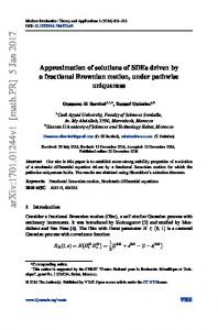
A comparison of computational complexity is presented in Figure 5.1. Figure 5.1a shows that both MC Picard I and MC Picard II are more expensive than the classical particle system. In Figure 5.1b, the iterated MLMC method is less expensive than the classical particle system method concerning the computational cost, as the mean-square-error bound ǫ2 decreases. Figure 5.1c illustrates that the error incurred from the iterated MLMC estimator is within 2ǫ of that of the classical particle system and that it decreases as number of particles increases. Moreover, Figure 5.2 confirms numerically that the iterated MLMC method can be improved by taking a decreasing sequence {ǫm }m=1,...,M , as opposed to taking a constant sequence. Finally, Figure 5.3 verifies, in the logarithm sense, the variance of PTi,m,ℓ for each Picard step. Also, it presents the logarithmic variance of PTi,m,ℓ − PTi,m,ℓ−1 . All lines of log2 Var[PTi,m,ℓ − PTi,m,ℓ−1 ] against ℓ have a slope of approximately −2 and this is higher than the rate given in Lemma 2.4, since it is well-known that for constant diffusion coefficients, the strong error of Euler scheme (2.4) is of order O(h−2 ℓ ).

40

18

260 Particle system MC Picard II MC Picard I

16

Particle system Iterated MLMC

240 220

14

Computational cost * ǫ 2

Computational cost *ǫ 3

200

12

10

8

6

180 160 140 120

4

100

2

0 0.005

80

0.006

0.007

0.008

0.009

0.01

0.011

0.012

Epsilon level (ǫ)

0.013

0.014

60 0.005

0.015

0.006

0.007

0.008

0.009

0.01

0.011

Epsilon level (ǫ)

0.012

0.013

0.014

0.015

(b) Iterated MLMC vs Particle method

(a) Iterated MC 0.08

MC Picard II vs Particle System MC Picard I vs Particle System Iterated MLMC vs Particle system Error upper bound (2ǫ) Error lower bound (-2 ǫ)

Difference against values of Particle system

0.06

0.04

0.02

0

-0.02

-0.04

-0.06

-0.08 1000

2000

3000

4000

5000

6000

7000

8000

9000

10000

Number of particles

(c) Approximation error

Figure 5.1: Comparison of computational complexity against ǫ 300

0.08 Iterated MLMC with ǫ 1>ǫ 2>...+ picard Iterated MLMC Particle system

Iterated MLMC with ǫ 1>ǫ 2>...+picard Iterated MLMC Upper error bound (2 ǫ) Lower error bound (-2 ǫ) zero difference

0.06

Difference against values of Particle system

Computational cost * ǫ 2

250

200

150

100

0.04

0.02

0

-0.02

-0.04

50 -0.06

0 0.005

0.006

0.007

0.008

0.009

0.01

0.011

Epsilon level (ǫ)

0.012

0.013

0.014

-0.08 1000

0.015

2000

3000

4000

5000

6000

7000

8000

Number of particles

(b) Approximation error

(a) Computational complexity against ǫ

Figure 5.2: Constant against a decreasing sequence

41

9000

10000

2 P 1l - P 1l-1 P 1l

0

P 2l - P 2l-1 P 2l

-2

P 3l - P 3l-1 P 3l

P 4l - P 4l-1

-4

log2 variance

P 4l

-6 -8 -10 -12 -14 -16 -18

0

1

2

3

4

5

6

7

8

level l

Figure 5.3: Variance of log2 against ℓ for all Picard steps

A Useful lemmas Lemma A.1. Let {Qt }t∈[0,T ] be a cadlag square-integrable process adapted to the filtration {Ft }t∈[0,T ] . Suppose that the Brownian motion {Wt }t∈[0,T ] is adapted to {Ft }t∈[0,T ] . Let G be a σ-algebra such that G ⊆ F0 . Then the following equalities hold for any t ∈ [0, T ].  Z t Qs dWs G = 0, (a) E 0  Z t  Z t 2  2 Qs ds G . Qs dWs G = E (b) E 0

0

Proof. (a) By the tower property of conditional expectation,     Z t Z t Qs dWs F0 G = 0. Qs dWs G = E E E 0

0

(b) Similarly, by Itô’s isometry and the tower property of conditional expectation,  Z t   Z t 2  2   Qs dWs G Qs dWs F0 G E = E E 0 0    Z t 2 Qs ds F0 G = E E 0  Z t 2 Qs ds G . = E 0

42

The following result concerning regular conditional probability distributions is needed in the proofs of Theorem 2.7 and Lemma 2.8. (For example, see Th.7.1 in [Parthasarathy, 1967] for details.) Lemma A.2. Let (M1 , B1 ) and (M2 , B2 ) be complete separable metric spaces. Let X and Y be random variables in the same probability space (Ω, F, P), with X taking values in (M1 , B1 ) and Y taking values in (M2 , B2 ). Let G ⊆ F be a sub σ-algebra. Suppose that Y is G-measurable. Then, for every Borel function h : M1 × M2 → R such that E|h(X, Y )| < +∞, there exists (a.s.) a probability measure µX|G : B1 × Ω → [0, 1] (called the regular conditional probability measure of X given G) such that Z
h(x, Y (ω)) µX|G (dx, ω). E[h(X, Y )|G] (ω) = M1

Suppose that, in addition, X is independent of G. Then, µX|G (·, ω) = Law(X) for ω-almost surely. ∗

Lemma A.3. The sequence {wm }M m=1 defined as ( ∗ −m−2)! max( (M , 1), M c ∗ −m−2 wm := 1,

m ≤ M∗ − 2 M∗ − 1 ≤ m ≤ M∗

satisfies properties (I) to (III). Proof. First, property (I) follows easily from the definition of it, since wm ≥ 1 = wM ∗ for all PM ∗ cM ∗ −m P ∗ cM ∗ −m values of m. For property (II), i.e. M m=1 (M ∗ −m)! wm & m=1 (M ∗ −m)! wm ∼ 1, we confirm that 1 by observing that ∗

∗

∗ ∗ MX −2 cM −m cM −m (M ∗ − m − 2)! w = max( , 1) + m ∗ (M ∗ − m)! (M ∗ − m)! cM −m−2 m=1 m=1

M X

M ∗ −2

&

X

m=1 M∗

=

X

∗

m=1

∗

cM −m + (M ∗ − m)!

X

m=M ∗ −1

∗

∗

m=M ∗ −1

∗

cM −m (M ∗ − m)!

cM −m (M ∗ − m)!

cM −m ∼ 1. ∗ − m)! (M m=1

Subsequently, we verify that M X

M∗

∗

M X

∗

PM ∗

∗

cM −m m=1 (M ∗ −m)! wm

. 1, since

∗ ∗ MX −2 cM −m cM −m (M ∗ − m − 2)! w = max( , 1) + m (M ∗ − m)! (M ∗ − m)! cM ∗ −m−2

m=1

43

∗

M X

m=M ∗ −1

∗

cM −m (M ∗ − m)!

.

∗ −2 MX

m=1

M∗

=

=

X

m=1 M∗ X

∗  cM −m  (M ∗ − m − 2)! + 1 + (M ∗ − m)! cM ∗ −m−2

=

M ∗ −2

m=1 ∗ −2 MX 2

M ∗ −m

c +c ∗ − m)! (M m=1 M X

m=1 M∗ X

∗

m=M ∗ −1

cM −m (M ∗ − m)!

X c c2 + (M ∗ − m)! (M ∗ − m)(M ∗ − m − 1)

∗

=

M ∗ −m

∗

M X

∗ cM −m

(M ∗

− m)!

+ c2

m=1 ∗ −1 MX

(

m=2

M ∗ −m

1 (M ∗ − m)(M ∗ − m − 1) 1 1 − ) m−1 m

c 1 + c2 (1 − ∗ ) ∼ 1. ∗ (M − m)! M −1 m=1

Lastly, we show this sequence has property (III). Since 0