ITERATIVE PROCEDURE FOR REAL SINGLE-TONE FREQUENCY ESTIMATION LIVIU TOMA, ALDO DE SABATA, ROBERT PAZSITKA
Keywords: Frequency estimation, Pisarenko harmonic decomposer, Filtering. We propose a simple, iterative procedure for the frequency estimation of a real sinusoid corrupted by additive, white noise, based on a combination of a known low-complexity method and filtering. We obtain mean square errors close to the Cramer-Rao lower bound, for relatively low signal-to-noise ratios in a few iterations, with a reasonable increase in computation complexity.
1. INTRODUCTION In many situations, a signal consisting of a single tone corrupted by additive white noise is available, and the frequency of the tone must be estimated. This problem has applications in communications, radar, sonar, measurements, adaptive control, speech processing etc [1], and it belongs to the wider class of spectrum estimation problems [2]. Both complex and real signals have been considered in the literature. As maximum likelihood (ML) estimators perform very well but are not computationally efficient [3, 4], various estimation algorithms have been proposed (see [5−11] for the complex case and [4, 12, 13, 14, 15] for the real case). The Pisarenko harmonic decomposer (PHD) [12, 13, 16, 17,], and the reformed Pisarenko harmonic decomposer (RPHD) [15, 18, 19] are among the algorithms that perform well and are computationally efficient in the real case, when the signal consists of a real sinusoid and an additive, white noise. The theory for both the above mentioned algorithms assumes a white noise. In the present paper we report an iterative method designed to improve the performance of the RPHD such that frequency error variances close to the Cramer-Rao lower bound (CRLB) are obtained for signal-to-noise ratios (SNR) as low as 3 dB in a few iterations. An iteration consists of filtering the initial data sequence with a frequency selective filter whose maximum of the frequency response is at the University Politehnica Timişoara, P-ţa Victoriei Nr. 2, 300006
[email protected],
[email protected],
[email protected]
Timişoara,
Rev. Roum. Sci. Techn. – Électrotechn. et Énerg., 54, 3, p. 253–259, Bucarest, 2009
România;
254
Liviu Toma, Aldo De Sabata, Robert Pazsitka
2
frequency estimate obtained in the previous iteration and in computing a better frequency estimate based on the data sequence at the filter output by means of the RPHD. Although the noise in the filtered sequence is no more white, experiments show that the considered estimators perform well in this case too. We present the algorithm in Section 2, together with an analysis of the increase in the SNR due to filtering. In Section 3 we report results of computer experiments, while conclusions are drawn in Section 4. 2. ITERATIVE PROCEDURE We consider the following signal model:
x ( n ) = s ( n ) + q ( n ) = α cos ( ω0 n + ϕ ) + q ( n ) , n = 1, 2,… , N
(1)
where α > 0 , ω0 ∈ (0, π) and ϕ are the deterministic but unknown amplitude, (angular) frequency and phase of the sinusoid respectively, and q(n) is a zero-mean Gaussian white noise of variance σ 2 . The signal-to-noise ratio is SNR 0 =
α2 . 2σ 2
(2)
In order to estimate the frequency we propose the following procedure: we initialize the algorithm by using the RPHD for the calculation of an initial estimate ˆ 0 for ω0 ; then we start iterations such that, at iteration k ≥ 1 , we filter the initial ω data sequence with a selective filter centered at the frequency estimated at iteration ˆ k −1 , and we apply to the signal from the filter output the RPHD in order to k–1, ω ˆk. calculate a new frequency estimate ω The purpose of filtering the data sequence is to increase the SNR. The filtered signal contains a colored noise component that does not fit into the theory of the frequency estimation algorithm we have mentioned, so that its performance has to be tested for this case. We have considered the second-order noise rejection filter with the following transfer function:
H ( z) =
z2 , z 2 − 2ρ cos(ω r ) z + ρ 2
(3)
where ρ is a parameter close to unity in order to provide selectivity (but smaller, for ˆ k −1 . stability) and, at each iteration k of the algorithm we have made ω r = ω
3
Iterative procedure for real single-tone frequency estimation
255
The performance of the noise-rejection filter can be illustrated by evaluating the enhancement η of the SNR η=
SNR1 , SNR 0
(4)
where SNR1=P1s/P1q is defined at the filter output and SNR0 has been defined in (2) (we have denoted by P1s and P1q the signal power and noise power at the filter output respectively). For evaluation purposes, we consider ω r = ω0 .
πA 2 [δ(ω − ω0 ) + δ(ω + ω0 )] and Pq (ω) = σ 2 the 2 power spectral densities of the signal and noise defined in (1) respectively, and by taking into account their statistical independence, we have Denoting further by Ps (ω) =
P1s =
1 2π
P1q =
1 2π
∫
π
∫
π
−π
−π
2
H (e jω ) Px (ω)d ω =
(
)
(5)
)
(6)
2(1 − ρ) 2 (1 + ρ) 2 − 4ρ cos 2 ω0
2
H (e jω ) Pq (ω)d ω =
α2
(
σ 2 (1 + ρ2 )
(1 − ρ2 ) ρ4 − 2ρ2 cos(2ω0 ) + 1
The integral in (5) is a simple application of the properties of the Dirac pulse, while the integral in (6) can be calculated in a straightforward way by means of the residuum theory. Simpler approximate expression are obtained by taking into account that ρ < 1, ρ ≅ 1 . The above results become: P1s ≅
α2 , 8(1 − ρ) 2 sin 2 ω 0
(7)
P1q ≅
σ2 . 4(1 − ρ) sin 2 ω 0
(8)
Finally, using (4), (7) and (8) we get η=
1 . 1− ρ
(9)
Equation (9) reveals an appreciable increase of the signal-to-noise ratio if we take into account the range of ρ ( ρ < 1, ρ ≅ 1) . These noise rejection properties of the filter and the fact that, due to the good estimation provided by the RPHD, the estimated frequency does not differ significantly from the true frequency are in
256
Liviu Toma, Aldo De Sabata, Robert Pazsitka
4
support of an iterative procedure that consists of computing k, k = 1, 2,… by using the signal at the filter output, with the previous estimate k–1 substituted for the parameter ω r in the expression of the frequency response. The variance of the estimator decreases at each iteration as the estimated frequency approaches gradually the true frequency. These a priori arguments are confirmed by experimental results presented in the next section. 3. SIMULATION RESULTS
frequency error [dB rad2]
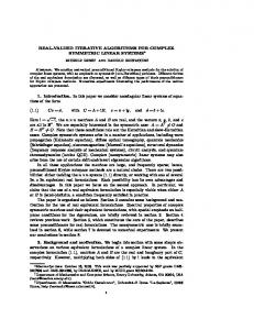
Computer experiments have been performed in order to evaluate the proposed iterative procedure. For frequency estimation, at each step of the algorithm we used the RPHD method [15]. The data sequence for single real, noisy sinusoids was generated using (1) with α = 2 and ϕ = 0 . We compared the estimates resulted from the iterative procedure after one iteration ( k = 1 ) and k = 5 iterations, to the RPHD method (corresponding to the initialization step of the algorithm) and to the CRLB [20]. The parameter ρ was chosen experimentally. The simulation results presented below are averages of 1000 independent runs. The results illustrated in Figs. 1, 2 and 3 indicate the decrease of the mean square frequency errors with the number of iterations. After five iterations, the estimator performance approaches the CRLB.
ω0/s Fig. 1 – Mean square frequency errors versus frequency for N = 50, SNR = 10 dB, ρ = 0.98.
Iterative procedure for real single-tone frequency estimation
257
frequency error [dB rad2]
5
ω0/s Fig. 2 – Mean square frequency errors versus frequency for N = 100, SNR = 3 dB, ρ = 0.95.
In experiments corresponding to Figs. 1 and 2, relatively low signal-to-noise ratios were chosen in order to prove the efficiency of the noise rejection filter. The larger SNR for the situation in Fig. 1 with respect to the one in Fig. 2 allowed for a smaller number of signal samples. Generally, a larger value of the SNR allows for a smaller number of signal samples and a value of ρ closer to 1 for achieving good estimates in a low number of iterations. Note that the frequency dependency of the mean square error, which occurs in real sinusoid frequency estimation, tends to decrease with the number of iterations. Experiment illustrated in Fig. 3 show that, at large SNR’s, the estimator performances approaches the CRLB after one iteration. The simulation results indicate that the desired performance of the algorithm is achieved in a few iterations. Consequently, the additional computation complexity introduced by iterations does not change the order of magnitude of the complexity of the original estimation method. In our examples, the RPHD (used at the initialization of the algorithm and then at each iteration) takes 3N–4 real multiplications, 4N–8 real additions and 5 other operation that are usually implemented by ROM accesses. Additionally, each iteration involves 2N–2 real multiplications and 2N–3 real additions for filtering and an RPHD. Therefore, for k iterations, the algorithm takes (5k+3)N–6k–4 real multiplications, (6K+4)N–11k–8 real additions and 5k+5 other operations. As shown above, a value of k = 5 is sufficient for achieving a good performance.
Liviu Toma, Aldo De Sabata, Robert Pazsitka
6
frequency error [dB rad2]
258
SNR [dB] Fig. 3 – Mean square frequency errors versus SNR, for f = 0.3, n = 100, ρ = 0.98.
4. CONCLUSIONS We have proposed an iterative algorithm for the estimation of the frequency of a signal consisting of a real sinusoid and an additive white noise. Starting from a known, single-step method (RPHD), we have used that method as a first step of the algorithm, then filtered the initial data sequence with a frequency selective filter centered on that estimate and used again that method on the filtered data in order to obtain the next estimate. This process has then been iterated. Filtering has been introduced in order to significantly improve the signal-tonoise ratio. Although after filtering the noise gets colored, experimental results show that the RPHD still provides good frequency estimates. Experiments indicate that this iterated procedure leads to an estimated frequency with a mean square error close to the CRLB, significantly improving the initial, first-step estimate in just a few iterations (below ten, tipically five). As the number of iterations is low, the asymptotic complexity of the algorithm is the same as in the initial method. Received on July 14, 2008
7
Iterative procedure for real single-tone frequency estimation
259
REFERENCES
1. P. Stoica, R. L. Moses, Introduction to Spectral Analysis, Prentice Hall, New Jersey, 1997. 2. S. M. Kay and S. L. Marple Jr., Spectrum Analysis – A Modern Perpective, Proc. of the IEEE, 69, 11, pp. 1360-1419, 1981. 3. D. C. Rife and R. R. Boorstyn, Single-Tone Parameter Estimation from Discrete-Time Observations, IEEE Trans. Inf. Theory, 20, 5, pp. 591-598, 1974. 4. R. J. Kenefic and A. H. Nuttall, Maximum Likelihood Estimation of the Parameters of a Tone Using Real Discrete Data, IEEE J. Oceanic Eng., OE-12, 1, pp. 279-280, 1987. 5. S. A. Tretter, Estimating the Frequency of a Noisy Sinusoid by Linear Regression, IEEE Trans. Inf. Theory, 31, 6, pp. 832-835, 1985. 6. S. A. Kay, A Fast and Accurate Single Frequency Estimator, IEEE Trans. ASSP, 37, 12, pp. 19871989, 1989. 7. M. P. Fitz, Further Results in the Fast Estimation of a Single Frequency, IEEE Trans. Comm., 42, 2/3/4, pp. 862-864, 1994. 8. M. Luise, R. Reggiannini, Carrier Frequency Recovery in All-Digital Modems for Burst-Mode Transmissions, IEEE Trans. Comm., 43, 2/3/4, pp. 1169-1178, 1995. 9. D. Kim, M. J. Narashima, An Improved Single Frequency Estimator, IEEE Signal Processing Letters, 3, 7, pp. 212-214, 1996. 10. E. Rosnes, A. Vahlin, Frequency Estimation of a Complex Sinusoid Using a Generalized Kay Estimator, IEEE Trans. Comm., 54, 3, pp. 407-415, 2006. 11. H. Fu, P. Y. Kam, MAP/ML Estimation of the Frequency and Phase of a single Sinusoid in Noise, IEEE Trans. Signal Processing., 55, 3, pp. 834-845, 2007. 12. H. Sakai, Statistical Analysis of Pisarenko's Method for Sinusoidal Frequency Estimation, IEEE Trans. ASSP, 32, 1, pp. 95-101, 1984. 13. K. W. Chan and H. C. So, An Exact Analysis of Pisarenko's Single-Tone Frequency Estimation Algorithm, Signal Processing, 83, pp. 685-690, 2003. 14. S. M. Savaresi, S. Bittanti, and H. C. So, Closed-Form, Unbiased Frequency Estimation of a Noisy Sinusoid Using Notch Filters, IEEE Trans. Aut. Control, 48, 7, pp. 1285-1292, 2003. 15. H. C. So and K. W. Chan, Reformulation of Pisarenko harmonic decomposition method for single-tone frequency estimation, IEEE Trans. Signal Process., 52, 4, pp. 1128–1135, April 2004. 16. V. F. Pisarenko, The retrieval of harmonics by linear prediction, Geophis, J. R. Astron. Soc., 33, pp. 347–366, 1973. 17. A. Eriksson and P. Stoica, On statistical analysis of Pisarenko tone frequency estimator, Signal Process., 31, 3, pp. 349–353, Apr. 1993. 18. H. C. So A closed form frequency estimator for a noisy sinusoid, 45th IEEE Midwest Symp. Circuits Systems, Tulsa, OK, 2002. 19. H. C. So and S. K. Ip, A novel frequency estimator and its comparative performances for short record lengths, 11th Eur. Signal Processing Conf., Toulouse, France, 2002. 20. S. M. Kay, Fundamentals of Statistical Signal Processing: Estimation Theory, Prentice Hall, New Jersey, 1993.
260
Liviu Toma, Aldo De Sabata, Robert Pazsitka
8