Apr 28, 2011 - arXiv:1104.5280v1 [stat.ML] 28 Apr 2011. ITERATIVE REWEIGHTED ALGORITHMS FOR SPARSE SIGNAL RECOVERY WITH. TEMPORALLY ...
ITERATIVE REWEIGHTED ALGORITHMS FOR SPARSE SIGNAL RECOVERY WITH TEMPORALLY CORRELATED SOURCE VECTORS
arXiv:1104.5280v1 [stat.ML] 28 Apr 2011
Zhilin Zhang and Bhaskar D. Rao Department of Electrical and Computer Engineering, University of California at San Diego, La Jolla, CA 92093-0407, USA {z4zhang,brao}@ucsd.edu ABSTRACT Iterative reweighted algorithms, as a class of algorithms for sparse signal recovery, have been found to have better performance than their non-reweighted counterparts. However, for solving the problem of multiple measurement vectors (MMVs), all the existing reweighted algorithms do not account for temporal correlation among source vectors and thus their performance degrades significantly in the presence of correlation. In this work we propose an iterative reweighted sparse Bayesian learning (SBL) algorithm exploiting the temporal correlation, and motivated by it, we propose a strategy to improve existing reweighted ℓ2 algorithms for the MMV problem, i.e. replacing their row norms with Mahalanobis distance measure. Simulations show that the proposed reweighted SBL algorithm has superior performance, and the proposed improvement strategy is effective for existing reweighted ℓ2 algorithms. Index Terms— Sparse Signal Recovery, Compressive Sensing, Iterative Reweighted ℓ2 Algorithms, Multiple Measurement Vectors, Sparse Bayesian Learning, Mahalanobis distance 1. INTRODUCTION The multiple measurement vector (MMV) model for sparse signal recovery is given by [1] Y = ΦX + V,
(1)
where Φ ∈ RN×M (N ≪ M ) is the dictionary matrix whose any N columns are linearly independent, Y ∈ RN×L is the measurement matrix consisting of L measurement vectors, X ∈ RM ×L is the source matrix with each row representing a possible source, and V is the white Gaussian noise matrix with each entry satisfying Vij ∼ N (0, λ). The key assumption under the MMV model is that the support (i.e. locations of nonzero entries) of every column vector X·i (∀i) 1 is identical (referred as the common sparsity assumption in the literature [1]). The MMV problem is often encountered in practical applications, such as neuroelectromagnetic source localization and direction-of-arrival estimation. Most algorithms for the MMV problem can be roughly divided into greedy methods, methods based on mixed norm optimization, iterative reweighted methods, and Bayesian methods. Iterative reweighted methods have received attention because of their improved performance compared to their non-reweighted counterparts [2, 3]. In [3], an iterative reweighted ℓ1 minimization framework is employed. The framework can be directly used for the MMV The work was supported by NSF Grant CCF-0830612. 1 The i-th column of X is denoted by X . The i-th row of X is denoted ·i by Xi· (also called the i-th source).
problem and many MMV algorithms based on mixed norm optimization can be improved via the framework. On the other hand, iterative reweighted ℓ2 algorithms were also proposed [2, 4]. The reweighted ℓ2 minimization framework for the MMV problem (in noisy case) computes the solution at the (k + 1)-th iteration as follows 2 : X (k) X(k+1) = arg min kY − ΦXk2F + λ wi (kXi· kq )2(2) x
i
=
W
(k)
Φ
T
λI + ΦW
(k)
(k)
Φ
T �−1
Y
(3)
where typically q = 2, W is a diagonal weighting matrix at the (k) (k) k-th iteration with i-th diagonal element being 1/wi , and wi depends on the previous estimate of X. Recently, Wipf et al [2] unified most existing iterative reweighted algorithms as belonging to the family of separable reweighted algorithms, whose weighting wi of a given row Xi· at each iteration is only a function of that individual row from the previous iteration. Further, they proposed nonseparable reweighted algorithms via variational approaches, which outperform many existing separable reweighted algorithms. In our previous work [5, 6] we showed that temporal correlation in sources Xi· seriously deteriorates recovery performance of existing algorithms and proposed a block sparse Bayesian learning (bSBL) framework, in which we incorporated temporal correlation and derived effective algorithms. These algorithms operate in the hyperparameter space, not in the source space as most sparse signal recovery algorithms do. Therefore, it is not clear what the connection of the bSBL framework is to other sparse signal recovery frameworks, such as the reweighted ℓ2 in (2). In this work, based on the cost function in the bSBL framework, we derive an iterative reweighted ℓ2 SBL algorithm with superior performance, which directly operates in the source space. Furthermore, motivated by the intuition gained from the algorithm and analytical insights, we propose a strategy to modify existing reweighted ℓ2 algorithms to incorporate temporal correlation of sources, and use two typical algorithms as illustrations. The strategy is shown to be effective. 2. THE BLOCK SPARSE BAYESIAN LEARNING FRAMEWORK The block sparse Bayesian learning (bSBL) framework [5, 6] transforms the MMV problem to a single measurement vector problem. This makes the modeling of temporal correlation much easier. First, we assume the rows of X are mutually independent, and the density of each row Xi· is multivariate Gaussian, given by p(Xi· ; γi , Bi ) ∼ N (0, γi Bi ),
i = 1, · · · , M
2 For convenience, we omit the superscript, k, on the right hand side of learning rules in the following.
where γi is a nonnegative hyperparameter controlling the row sparsity of X as in the basic sparse Bayesian learning [7, 8]. When γi = 0, the associated i-th row of X becomes zero. Bi is an unknown positive definite correlation matrix. By letting y = vec(Y T ) ∈ RNL×1 , D = Φ ⊗ IL 3 , x = vec(XT ) ∈ RM L×1 and v = vec(VT ), where vec(A) denotes the vectorization of the matrix A formed by stacking its columns into a single column vector, we can transform the MMV model (1) to the block single vector model as follows y = Dx + v.
(4)
To elaborate on the block sparsity model (4), we rewrite PMit as y = [Φ1 ⊗ IL , · · · , ΦM ⊗ IL ][xT1 , · · · , xTM ]T + v = i=1 (Φi ⊗ IL )xi + v, where Φi is the i-th column of Φ, xi ∈ RL×1 is the i-th block in x and it is the transposed i-th row of X in the original MMV model (1), i.e. xi = XTi· . K nonzero rows in X means K nonzero blocks in x. Thus we refer to x as block-sparse. For the block model (4), the Gaussian likelihood is p(y|x; λ) ∼ Ny|x (Dx, λI). The prior for x is given by p(x; γi , Bi , ∀i) ∼ Nx (0, Σ0 ), where Σ0 is a block diagonal matrix with the ith diagonal block γi Bi (∀i). Given the hyperparameters Θ , {λ, γi , Bi , ∀i}, the Maximum A Posterior (MAP) estimate of x can be directly obtained from the posterior of the model. To estimate these hyperparameters, we can use the Type-II maximum likelihood method [8], which marginalizes over x and then performs maximum likelihood estimation, leading to the cost function: Z L(Θ) , −2 log p(y|x; λ)p(x; γi , Bi , ∀i)dx =
log |λI + DΣ0 DT | + yT (λI + DΣ0 DT )−1 y,(5)
where γ , [γ1 , · · · , γM ]T . We refer to the whole framework including the solution estimation of x and the hyperparameter estimation as the bSBL framework. Note that in contrast to the original SBL framework, the bSBL framework models the temporal correlation structure of sources in the prior density via the matrix Bi (∀i). 3. ITERATIVE REWEIGHTED SPARSE BAYESIAN LEARNING ALGORITHMS Based on the cost function (5), we can derive efficient algorithms that exploit temporal correlation of sources [5, 6]. But these algorithms directly operate in the hyperparameter space (i.e. the γ-space). So, it is not clear what their connection is to other sparse signal recovery algorithms that directly operate in the source space (i.e. the Xspace) by minimizing penalties on the sparsity of X. Particularly, it is interesting to see if we can transplant the benefits gained from the bSBL framework to other sparse signal recovery frameworks such as the iterative reweighted ℓ2 minimization framework (2), improving algorithms belonging to those frameworks. Following the approach developed by Wipf et al [2] for the single measurement vector problem, in the following we use the duality theory [9] to obtain a penalty in the source space, based on which we derive an iterative reweighted algorithm for the MMV problem. 3.1. Algorithms First, we find that assigning a different covariance matrix Bi to each source Xi· will result in overfitting in the learning of the hyperpa3 We denote the L × L identity matrix by I . When the dimension is L evident from the context, for simplicity we use I. ⊗ is the Kronecker product.
rameters. To overcome the overfitting, we simplify and consider using one matrix B to model all the source covariance matrixes. Thus Σ0 = Γ ⊗ B with Γ , diag([γ1 , · · · , γM ]). Simulations will show that this simplification leads to good results even if different sources have different temporal correlations (see Section 5). In order to transform the cost function (5) to the�source space, we use the identity: yT (λI + DΣ0 DT )−1 y ≡ minx λ1 ky − Dxk22 + � xT Σ−1 0 x , by which we can upper-bound the cost function (5) and obtain the bound 1 L(x, γ, B) = log |λI + DΣ0 DT | + ky − Dxk22 + xT Σ−1 0 x. λ By first minimizing over γ and B and then minimizing over x, we can get the cost function in the source space: x = arg min ky − Dxk22 + λgTC (x), x
(6)
where the penalty gTC (x) is defined by gTC (x) ,
min
γ�0,B≻0
T xT Σ−1 0 x + log |λI + DΣ0 D |.
(7)
From the definition (7) we have gTC (x)
≤ = ≤
T xT Σ−1 0 x + log |λI + DΣ0 D | 1 T −1 xT Σ−1 0 x + log |Σ0 | + log | D D + Σ0 | + N L log λ λ T −1 xT Σ−1 − f ∗ (z) + N L log λ 0 x + log |Σ0 | + z γ
where in the last inequality we have used the conjugate relation 1 = min zT γ −1 − f ∗ (z). (8) log DT D + Σ−1 0 z�0 λ
−1 T Here we denote γ −1 , [γ1−1 , · · · , γM ] , z , [z1 , · · · , zM ]T , and ∗ −1 f (z) is concave conjugate of f (γ ) , log | λ1 DT D + Σ−1 0 |. Finally, reminding of Σ0 = Γ ⊗ B, we have
gTC (x) ≤
N L log λ − f ∗ (z) + M log |B| + M h T −1 i X x i B x i + zi + L log γi . γi i=1
(9)
Therefore, to solve the problem (6) with (9), we can perform the coordinate descent method over x, B, z and γ, i.e, min
x,B,z�0,γ�0
M � T −1 hX x i B x i + zi γi i=1 � i (10) +L log γi + M log |B| − f ∗ (z) .
ky − Dxk22 + λ
Compared to the framework (2), we can see 1/γi can be seen as the weighting for the corresponding xTi B−1 xi . But instead of applying ℓq norm on xi (i.e. the i-th row of X) as done in existing iterative reweighted ℓ2 algorithms, our algorithm computes xTi B−1 xi , i.e. the quadratic Mahalanobis distance of xi and its mean vector 0. By minimizing (10) over x, the updating rule for x is given by x(k+1) = Σ0 DT (λI + DΣ0 DT )−1 y.
(11)
According to the dual property [9], from the relation (8), the optimal z is directly given by zi
= =
∂ log | λ1 DT D + Σ−1 0 | ∂(γi−1 ) h �−1 i Lγi − γi2 Tr BDTi λI + DΣ0 DT Di , ∀i (12)
where Di consists of columns of D from the ((i − 1)L + 1)-th to the (iL)-th. From (10) the optimal γi for fixed x, z, B is given by γi = L1 [xTi B−1 xi + zi ]. Substituting Eq.(12) into it, we have xTi B−1 xi + γi L h 2 �−1 i γ − i Tr BDTi λI + DΣ0 DT Di , ∀i (13) L By minimizing (10) over B, the updating rule for B is given by (k+1)
γi
=
B(k+1) = B/kBkF ,
with
B=
M X xi xTi i=1
γi
.
(14)
The updating rules (11) (13) and (14) are our reweighted algorithm minimizing the penalty based on quadratic Mahalanobis distance of xi . Since for a given i, the weighting 1/γi depends on the whole estimated source matrix in the previous iteration (via B and Σ0 ), the algorithm is a nonseparable reweighted algorithm. The complexity of this algorithm is high because it learns the parameters in a higher dimensional space than the original problem space. For example, consider the bSBL framework, in which the dictionary matrix D is of the size N L × M L, while in the original MMV model the dictionary matrix is of the size N × M . We use an approximation to simplify the algorithm and develop an efficient variant. Using the approximation: �−1 �−1 λINL + DΣ0 DT ≈ λIN + ΦΓΦT ⊗ B−1 , (15) which takes the equal sign when λ = 0 or B = I, the updating rule (11) can be transformed to �−1 X(k+1) = WΦT λI + ΦWΦT Y, (16)
where W , diag([1/w1 , · · · , 1/wM ]) with wi , 1/γi . Using the same approximation, the last term in (13) becomes h �−1 i Tr BDTi λINL + DΣ0 DT Di i h � � ≈ Tr B(ΦTi ⊗ I) (λIN + ΦWΦT )−1 ⊗ B−1 (Φi ⊗ I) = LΦTi (λIN + ΦWΦT )−1 Φi .
Therefore, from the updating rule of γi (13) we have h1 i−1 1 (k+1) wi = . (17) Xi· B−1 XTi· + {(W−1 + ΦT Φ)−1 }ii L λ Accordingly, the updating rule for B becomes B(k+1) = B/kBkF ,
with
B=
M X
wi XTi· Xi· .
(18)
i=1
We denote the updating rules (16) (17) and (18) by ReSBL-QM. With the aid of singular value decomposition, the computational complexity of the algorithm is O(N 2 M ) (The effect of L can be removed by using the strategy in [7]). 3.2. Estimate the Regularization Parameter λ To estimate the regularization parameter λ, many methods have been proposed, such as the modified L-curve method [1]. Here, straightforwardly following the Expectation-Maximization method in [5] and using the approximation (15), we derive a learning rule for λ, given by: � λ � 1 kY − ΦXk2F + Tr G(λI + G)−1 . λ(k+1) = NL N where G , ΦWΦT .
3.3. Theoretical Analysis in the Noiseless Case For the noiseless inverse problem Y = ΦX, denote the generating sources by Xgen , which is the sparsest solution among all the possible solutions. Assume Xgen is full column-rank. Denote the true source number (i.e. the true number of nonzero rows in Xgen ) by K0 . Now we have the following result on the global minimum of the cost function (5): Theorem 1 In the noiseless case, assuming K0 < (N + L)/2, for the cost function (5) the unique global minimum γ b = b that equals to Xgen [b γ1 , · · · , b γM ] produces a source estimate X b i , ∀i, where X b is obtained from irrespective of the estimated B bT) = x b and x b is computed using Eq.(11). vec(X The proof is given in [6]. The theorem implies that even if the b i is different from the true Bi , the estimated sources are estimated B the true sources at the global minimum of the cost function. Thereb i does not harm the recovery of true fore the estimation error in B sources. As a reminder, in deriving our algorithm, we assumed Bi = B (∀i) to avoid overfitting. The theorem ensures that this strategy does not harm the global minimum property. In our work [6] we have shown that B plays the role of whitening sources in the SBL procedure, which can be seen in our algorithm as well. This gives us a motivation to improve some state-of-the-art reweighted ℓ2 algorithms by whitening the estimated sources in their weighting rules and penalties, detailed in the next section. 4. MODIFY EXISTING REWEIGHTED ℓ2 METHODS Motivated by the above results and our analysis in [6], we can modify many reweighted ℓ2 algorithms via replacing the ℓ2 norm of Xi· by some suitable function of its Mahalanobis distance. Note that similar modifications can be applied on reweighted ℓ1 algorithms. The regularized M-FOCUSS [1] is a typical reweighted ℓ2 algorithm, which solves a reweighted ℓ2 minimization with weights (k) (k) wi = (kXi· k22 )p/2−1 in each iteration. It is given by �−1 X(k+1) = W(k) ΦT λI + ΦW(k) ΦT Y (19) W(k)
=
(k)
=
wi
(k)
(k)
diag{[1/w1 , · · · , 1/wM ]} �p/2−1 (k) kXi· k22 , p ∈ [0, 2], ∀i
(20)
We can modify the algorithm by changing (20) to the following one: �p/2−1 (k) (k) (k) wi = Xi· (B(k) )−1 (Xi· )T , p ∈ [0, 2], ∀i (21)
The matrix B can be calculated using the learning rule (18). We denote the modified algorithm by tMFOCUSS. In [4] Chartrand and Yin proposed an iterative reweighted ℓ2 algorithm based on the classic FOCUSS algorithm. Its MMV extension (denoted by Iter-L2) changed (20) to: �p/2−1 (k) (k) , p ∈ [0, 2], ∀i (22) wi = kXi· k22 + ǫ Their algorithm adopts the strategy: initially use a relatively large ǫ, then repeating the process of decreasing ǫ after convergence and repeating the iteration (19), dramatically improving the recovery ability. Similarly, we can modify the weighting (22) to the following rule incorporating the temporal correlation of sources: �p/2−1 (k) (k) (k) wi = Xi· (B(k) )−1 (Xi· )T + ǫ , p ∈ [0, 2], ∀i (23)
and adopts the same ǫ-decreasing strategy. B is also given by (18). We denote the modified algorithm by tIter-L2.
5. EXPERIMENTS
4 Since in our experiments the measurement vector number is very small (L = 3 or 4), generating sources as AR(1) with various AR coefficient values is sufficient.
0.6
0.8
Failure Rate
Failure Rate
0.8
1
ReSBL−QM ReSBL−L2 tMFOCUSS MFOCUSS tIter−L2 Iter−L2 Iter−L1
0.4
0 10
0.6
0.4
0.2
0.2
12 14 Number of Nonzero Sources K
(a) Low Correlation Case
16
0 10
12 14 Number of Nonzero Sources K
0.6
0.8
Failure Rate
0.8
1
ReSBL−QM ReSBL−L2 tMFOCUSS MFOCUSS tIter−L2 Iter−L2 Iter−L1
0.4
16
(b) High Correlation Case
Fig. 1. Performance when the nonzero source number changes.
0
0.6
0.4
0.2
0.2
In our experiments, a dictionary matrix Φ ∈ RN×M was created with columns uniformly drawing from the surface of a unit hypersphere. The source matrix Xgen ∈ RM ×L was randomly generated with K nonzero rows of unit norms, whose row locations were randomly chosen. Amplitudes of the i-th nonzero row were generated as an AR(1) process whose AR coefficient was denoted by βi 4 . Thus βi indicates the temporal correlation of the i-th source. The measurement matrix was constructed by Y = ΦXgen + V, where V was a zero-mean homoscedastic Gaussian noise matrix with variance adjusted to have a desired value of SNR. For each different experiment setting, we repeated 500 trials and averaged results. The performance measurement was the Failure Rate defined in [7], which indicated the percentage of failed trials in the 500 trials. When noise was present, since we could not expect any algorithm to recover Xgen exactly, we classified a trial as a failure trial if the K largest estimated row-norms did not align with the support of Xgen . The compared algorithms included our proposed ReSBL-QM, tMFOCUSS, tIter-L2, the reweighted ℓ2 SBL in [2] (denoted by ReSBL-L2), M-FOCUSS [1], Iter-L2 presented in Section 4, and Candes’ reweighted ℓ1 algorithm [3] (extended to the MMV case as suggested by [2], denoted by Iter-L1). For tMFOCUSS, M-FOCUSS, and Iter-L2, we set p = 0.8, which gave the best performance in our simulations. For Iter-L1, we used 5 iterations. In the first experiment we fixed N = 25, M = 100, L = 3 and SNR = 25dB. The number of nonzero sources K varied from 10 to 16. Fig.1 (a) shows the results when each βi was uniformly chosen from [0, 0.5) at random. Fig.1 (b) shows the results when each βi was uniformly chosen from [0.5, 1) at random. In the second experiment we fixed N = 25, L = 4, K = 12, and SNR = 25dB, while M/N varied from 1 to 25. βi (∀i) in Fig.2 (a) and (b) were generated as in Fig.1 (a) and (b), respectively. This experiment aims to see algorithms’ performance in highly underdetermined inverse problems, which met in some applications such as neuroelectromagnetic source localization. From the two experiments we can see that: (a) in all cases, the proposed ReSBL-QM has superior performance to other algorithms,
1
1
Failure Rate
The proposed tMFOCUSS and tIter-L2 have convergence properties similar to M-FOCUSS and Iter-L2, respectively. Due to space limit we omit theoretical analysis, and instead, provide some representative simulation results in the next section.
5
10
15
20
M/N
25
0
5
10
15
20
25
M/N
(a) Low Correlation Case
(b) High Correlation Case
Fig. 2. Performance when M/N changes. capable to recover more sources and solve more highly underdetermined inverse problems; (b) without considering temporal correlation of sources, existing algorithms’ performance significantly degrades with increasing correlation; (c) after incorporating the temporal structures of sources, the modified algorithms, i.e. tMFOCUSS and tIter-L2, have better performance than the original M-FOCUSS and Iter-L2, respectively. Also, we noted that our proposed algorithms are more effective when the norms of sources have no large difference (results are not shown here due to space limit). 6. CONCLUSIONS In this paper, we derived an iterative reweighted sparse Bayesian algorithm exploiting the temporal structure of sources. Its simplified variant was also obtained, which has less computational load. Motivated by our analysis we modified some state-of-the-art reweighted ℓ2 algorithms achieving improved performance. This work not only provides some effective reweighted algorithms, but also provides a strategy to design effective reweighted algorithms enriching current algorithms on this topic. 7. REFERENCES [1] S. F. Cotter and B. D. Rao, “Sparse solutions to linear inverse problems with multiple measurement vectors,” IEEE Trans. on Signal Processing, vol. 53, no. 7, 2005. [2] D. Wipf and S. Nagarajan, “Iterative reweighted ℓ1 and ℓ2 methods for finding sparse solutions,” IEEE Journal of Selected Topics in Signal Processing, vol. 4, no. 2, 2010. [3] E. J. Candes and et al, “Enhancing sparsity by reweighted ℓ1 minimization,” J Fourier Anal Appl, vol. 14, 2008. [4] R. Chartrand and W. Yin, “Iteratively reweighted algorithms for compressive sensing,” in ICASSP 2008. [5] Z. Zhang and B. D. Rao, “Sparse signal recovery in the presence of correlated multiple measurement vectors,” in ICASSP 2010. [6] ——, “Sparse signal recovery with temporally correlated source vectors using sparse Bayesian learning,” IEEE Journal of Selected Topics in Signal Processing, submitted. [7] D. P. Wipf and B. D. Rao, “An empirical Bayesian strategy for solving the simultaneous sparse approximation problem,” IEEE Trans. on Signal Processing, vol. 55, no. 7, 2007. [8] M. E. Tipping, “Sparse Bayesian learning and the relevance vector machine,” J. Mach. Learn. Res., vol. 1, pp. 211–244, 2001. [9] S. Boyd and L. Vandenberghe, Convex Optimization. Cambridge University Press, 2004.