Each step of this algorithm uses the full sample of four- tuples gathered from interaction ... to allow the use of standard batch mode supervised learning algorithms, instead of the ..... 3 Illustration: âCar on the Hillâ Control Problem. The precise ...
Iteratively Extending Time Horizon Reinforcement Learning Damien Ernst� , Pierre Geurts�� , and Louis Wehenkel Department of Electrical Engineering and Computer Science Institut Montefiore, University of Li`ege Sart-Tilman B28, B4000 Li`ege, Belgium {ernst,geurts,lwh}@montefiore.ulg.ac.be
Abstract. Reinforcement learning aims to determine an (infinite time horizon) optimal control policy from interaction with a system. It can be solved by approximating the so-called Q-function from a sample of four-tuples (xt , ut , rt , xt+1 ) where xt denotes the system state at time t, ut the control action taken, rt the instantaneous reward obtained and xt+1 the successor state of the system, and by determining the optimal control from the Q-function. Classical reinforcement learning algorithms use an ad hoc version of stochastic approximation which iterates over the Q-function approximations on a four-tuple by four-tuple basis. In this paper, we reformulate this problem as a sequence of batch mode supervised learning problems which in the limit converges to (an approximation of) the Q-function. Each step of this algorithm uses the full sample of fourtuples gathered from interaction with the system and extends by one step the horizon of the optimality criterion. An advantage of this approach is to allow the use of standard batch mode supervised learning algorithms, instead of the incremental versions used up to now. In addition to a theoretical justification the paper provides empirical tests in the context of the “Car on the Hill” control problem based on the use of ensembles of regression trees. The resulting algorithm is in principle able to handle efficiently large scale reinforcement learning problems.
1
Introduction
Many interesting problems in many fields can be formulated as closed-loop control problems, i.e. problems whose solution is provided by a mapping (or a control policy) ut = µ(xt ) where xt denotes the state at time t of a system and ut an action taken by a controlling agent so as to influence the instantaneous and future behavior of the system. In many cases these problems can be formulated as infinite horizon discounted reward discrete-time optimal control problems, i.e. problems where the objective is to find a (stationary) control policy µ∗ (·) which maximizes the expected return over an infinite time horizon defined as follows: � ��
Research Fellow FNRS Postdoctoral Researcher FNRS
N. Lavraˇ c et al. (Eds.): ECML 2003, LNAI 2837, pp. 96–107, 2003. c Springer-Verlag Berlin Heidelberg 2003 �
Iteratively Extending Time Horizon Reinforcement Learning µ J∞
= lim E
�N −1 �
N →∞
97
� t
γ rt
,
(1)
t=0
where γ ∈ [0, 1[ is the discount factor, rt is an instantaneous reward signal which depends only on the state xt and action ut at time t, and where the expectation is taken over all possible system trajectories induced by the control policy µ(·). Optimal control theory, and in particular dynamic programming, aims to solve this problem “exactly” when the explicit knowledge of system dynamics and reward function are given a priori. In this paper we focus on reinforcement learning (RL), i.e. the use of automatic learning algorithms in order to solve the optimal control problem “approximately” when the sole information available is the one we obtain from system transitions from t to t+1. Each system transition provides the knowledge of a new four-tuple (xt , ut , rt , xt+1 ) of information and we aim here to compute µ∗ (.) from a sample F = (xkt , ukt , rtk , xkt+1 ), k = 1, . . . , � of such four-tuples. It is important to contrast the RL protocol with the standard batch mode supervised learning protocol, which aims at determining, from the sole information of a sample S of input-output pairs (i, o), a function h∗ ∈ H (H is called the hypothesis space of the learning algorithm) which minimizes the expected approximation error, e.g. defined in the case of least squares regression by the following functional: � Errh = |h(i) − o|2 . (2) (i,o)∈S
Notice that the use of supervised learning in the context of optimal control problems would be straightforward if, instead of the sample F of four-tuples, we could provide the learning algorithm with a sample of input-output pairs (x, µ∗ (x)) (see for example [9] for a discussion on the combination of such a scheme with reinforcement learning). Unfortunately, in many interesting control problems this type of information can not be acquired directly, and the specific difficulty in reinforcement learning is to infer a good approximation of the optimal control policy only from the information given in the sample F of four-tuples. Existing reinforcement learning algorithms can be classified into two categories: – Model based RL methods: they use (batch mode or incremental mode) supervised learning to determine from the sample F of four-tuples on the one hand an approximation of the system dynamics: f1 (x, u, x� ) ≈ P (xt+1 = x� |xt = x, ut = u)
(3)
and on the other hand an approximation of the expected reward function: f2 (x, u) ≈ E{rt |xt = x, ut = u}.
(4)
Once these two functions have been obtained, model based algorithms derive the optimal control policy by dynamic programming [5, 8].
98
Damien Ernst, Pierre Geurts, and Louis Wehenkel
– Non-model based RL methods: they use incremental mode supervised learning in order to determine an approximation of the Q-function associated to the control problem. This function is (implicitly) defined by the following equation (known as the Bellman equation): � � � � � Q(x, u) = E rt + γmax Q(x , u ) x = x, u = u . (5) � t+1 t t � u
The optimal control policy can be directly determined from this (unique) Q-function by the following relation µ∗ (x) = arg maxQ(x, u). u
(6)
The most well-known algorithm falling into the latter category is the socalled Q-learning method [11]. Our proposal is based on the observation that neither of these two approaches are able to fully exploit the power of modern supervised learning methods. Indeed, model based approaches are essentially linked to so-called state space discretization which aims at building a finite Markov Decision Problem (MDP) and are strongly limited by the curse of dimensionality: in order to use the dynamic programming algorithms, the state and control spaces need to be discretized and the number of cells of any discretization scheme increases exponentially with the number of dimensions of the state space. Non-model based approaches have, to our best knowledge, been combined only with incremental (on-line) learning algorithms (see e.g. [10]). With respect to these approaches, we propose a novel non-model based RL framework which is able to exploit any generic batch mode supervised learning algorithm to model the Q-function. The resulting algorithm is illustrated on a simple problem where it is combined with three supervised learning algorithms based on regression trees. The rest of the paper is organized as follows: Section 2 introduces the underlying idea of our approach and gives a precise description of the proposed algorithm; Section 3 provides a validation in the context of the “Car on the Hill” control problem; Section 4 provides discussions, directions for future research and conclusions.
2
Iteratively Extending Time Horizon in Optimal Control
The approach that we present is based on the fact that the optimal (stationary) control policy of an infinite horizon problem can be formalized as the limit of a sequence of finite horizon control problems, which can be solved in an iterative fashion by using any standard supervised learning algorithm. 2.1
Iteratively Extending time Horizon in Dynamic Programming
We consider a discrete-time stationary stochastic system defined by its dynamics, i.e. a transition function defined over the Cartesian product X × U × W of the state space X, the control space U , and the disturbance space W : xt+1 = f (xt , ut , wt ),
(7)
Iteratively Extending Time Horizon Reinforcement Learning
99
a reward signal also defined over X × U × W : rt = r(xt , ut , wt ),
(8)
a noise process defined by a conditional probability distribution: wt ∼ Pw (w = wt |x = xt , u = ut ),
(9)
and a probability distribution over the initial conditions: x0 ∼ Px (x = x0 ).
(10)
For a given (finite) horizon N , let us denote by πN (t, x) ∈ U, t ∈ {0, . . . , N − 1}; x ∈ X
(11)
a (possibly time varying) N -step control policy (i.e. ut = πN (t, xt )), and by πN JN = E{
N −1 �
γ t rt }
(12)
t=0
the N -step reward of the closed-loop system using this policy. An N -step optimal πN policy is a policy which among all possible such policies maximizes JN for any Px on the initial conditions. Notice that (under mild conditions) such a policy always does indeed exist although it is not necessarily unique. Our algorithm exploits the following properties of N -step optimal policies (these are classical results of dynamic programming theory [1]): 1. The sequence of policies obtained by considering the sequence of Qi -functions iteratively defined by Q1 (x, u) = E{rt |xt = x, ut = u} and QN (x, u) = E
�
(13)
� � � � rt + γmax Q (x , u ) x = x, u = u , ∀N > 1, (14) � N −1 t+1 t t � u
and the following two conditions1 ∗ πN (0, x) = arg maxQN (x, u), ∀N ≥ 0
(15)
∗ ∗ (t + 1, x) = πN πN −1 (t, x), ∀N > 1, t ∈ {0, . . . , N − 2}
(16)
u
and
is optimal. ∗ 2. The sequence of stationary policies defined by µ∗N (x) = πN (0, x) converges ∗ (globally, and for any Px on the initial conditions) to µ (x) in the sense that µ∗
∗
µ . lim J∞N = J∞
N →∞
(17)
3. The sequence of functions QN converges to the (unique) solution of the Bellman equation (eqn. (5)). 1
Actually this definition does not necessarily yield a unique policy, but any policy which satisfies this condition is appropriate, and it is straightforward to define a procedure constructing such a policy from the sequence of Qi -functions.
100
2.2
Damien Ernst, Pierre Geurts, and Louis Wehenkel
Iteratively Extending Time Horizon in Reinforcement Learning
The proposed algorithm is based on the use of supervised learning in order to ˆ i of approximations of the Qi -functions defined above, by produce a sequence Q exploiting at each step the full sample of four-tuples F = (xkt , ukt , rtk , xkt+1 ), k = 1, . . . , � in batch mode together with the function produced at the preceding step. Initialization. The algorithm starts by using the sample F of four-tuples in order to construct an approximation of Q1 (x, u). This can be achieved using the xt , ut components of each four-tuple as inputs, and the rt component as output and by using a supervised regression algorithm in order to find in its hypothesis space H a function satisfying ˆ 1 = arg min Q h∈H
� �
|h(xkt , ukt ) − rtk |2 .
(18)
k=1
Iteration. Step i (i > 1) of the algorithm uses the function produced at step i−1 to modify the output of each input-output pair associated to each four-tuple by ˆ i−1 (xkt+1 , u� ) oki = rtk + γmax (19) Q � u
and then applies the supervised learning algorithm to build ˆ i = arg min Q h∈H
� �
|h(xkt , ukt ) − oki |2 .
(20)
k=1
Stopping Conditions. For the theoretical sequence of policies an error bound on the sub-optimality in terms of the number of iterations is given by the following equation γ N Br µ∗ µ∗ , (21) |J∞N − J∞ |< 1−γ where Br > sup r(x, u, w). This equation can be used to fix an upper bound on the number of iterations for a given a priori fixed optimality gap. Another possibility is to exploit the convergence property of the sequence of Qi -functions in order to decide when to stop the iteration, e.g. when ˆN − Q ˆ N −1 | < �. |Q
(22)
Control Policy Derivation. The final control policy seen as an approximation of the optimal stationary closed-loop policy is in principle derived by ˆ N (x, u). µ ˆ∗ (x) = µ ˆ∗N (x) = arg maxQ u
(23)
If the control space is finite, this can be done using exhaustive search. Otherwise, the algorithm to achieve this will depend on the type of approximation architecture used.
Iteratively Extending Time Horizon Reinforcement Learning
101
Consistency. It is interesting to question under which conditions this algorithm provides consistency, i.e. under which conditions the sequence of policies generated by our algorithm and using a sample of increasing size would converge to the optimal control policy within a pre-specified optimality gap. Without any assumption on the used supervised learning algorithm and on the sampling mechanism nothing can be said about consistency. On the other hand, if each one of the true Qi -functions can be arbitrarily well approximated by a function of the hypothesis space and if the sample (in asymptotic regime) contains an infinite number of times each possible state-action pair (x, u), then consistency is ensured trivially. Further research is necessary in order to determine less ideal assumptions both on the hypothesis space and on the sampling mechanism which would still guarantee consistency. Solution Characterization. Another way to state the reinforcement learning problem would consist of defining the approximate Q-function as the solution of the following equation ˆ = arg min Q h∈H
l � � ��2 � � k � � h(x , u ) �h(xkt , ukt ) − rtk + γmax � . t+1 � u
k=1
(24)
Our algorithm can be viewed as an iterative algorithm to solve this minimization problem starting with an initial guess Q0 (x, u) ≡ 0 and at each iteration i > 0 updating the function according to ˆ i = arg min Q h∈H
2.3
l � � ��2 � � ˆ i−1 (xkt+1 , u� ) �� . Q �h(xkt , ukt ) − rtk + γmax �
k=1
u
(25)
Supervised Regression Algorithm
In principle, the proposed framework can be combined with any available supervised learning method designed for regression problems. In order to be practical, the desirable features of the used algorithm are as follows: – Computational efficiency and scalability of the learning algorithm. Specially with respect to sample size and dimensionality of the state space X and the control space U . – Modeling flexibility. The Qi -functions to be modeled by the algorithm are unpredictable in shape; hence no prior assumption can be made on the parametric shape of the approximation architecture, and the automatic learning algorithm should be able to adapt its model by itself to the problem data. – Reduced variance, in order to work efficiently in small sample regimes. – Fully automatic operation. The algorithm may be called several hundred times and it is therefore not possible to ask for a human operator to tune some meta-parameters at each step of the iterative procedure. – Efficient use of the model, in order to derive the control from the Q-function.
102
Damien Ernst, Pierre Geurts, and Louis Wehenkel
In the simulation results given in the next section, we have compared three learning algorithms based on regression trees which we think offer a good compromise in terms of the criteria established above. We give a very brief description of each variant below. Regression Trees. Classification and regression trees are among the most popular supervised learning algorithms. They combine several characteristics such as interpretability of the models, efficiency, flexibility, and fully automatic operation which make them particularly attractive for this application. To build such trees, we have implemented the CART algorithm as described in [4]. Tree Bagging. One drawback of regression trees is that they suffer from a high variance. Bagging [2] is an ensemble method proposed by Breiman that often improves very dramatically the accuracy of trees by reducing their variance. With bagging, several regression trees are built, each from a different bootstrap sample drawn from the original learning sample. To make a prediction with this set of M trees, we simply take the average predictions of these M trees. Note that, while bagging inherits several advantages of regression trees, it increases their computing times significantly. Extremely Randomized Trees (Extra-trees). Besides bagging, several other methods to build tree ensembles have been proposed that often improve the accuracy with respect to tree bagging (e.g. random forests [3]). In this paper, we propose to evaluate our own recent proposal which is called “Extra-trees”. Like bagging, this algorithm works by taking the average predictions of several trees. Each of these trees is built from the the original learning sample by selecting its tests fully at random. The main advantages of this algorithm with respect to bagging is that it is computationally much faster (because of the extreme randomization) and also often more accurate. For more details about this algorithm, we refer the interested reader to [6, 7].
3
Illustration: “Car on the Hill” Control Problem
The precise definition of the test problem is given in the appendix. It is a version of a quite classical test problem used in the reinforcement learning literature. A car is traveling on a hill (the shape of which is given by the function H(p) of Figure 3b). The objective is to bring the car in minimal time to the top of the hill (p = 1 in Figure 3b). The problem is studied in discrete-time, which means here that the control variable can be changed only every 0.1 s. The control variable acts directly on the acceleration of the car (eqn. (27), appendix) but can only assume two extreme values (full acceleration or full deceleration). The reward signal is defined in such a way that the infinite horizon optimal control policy is a minimum time control strategy (eqn. (29), appendix). Our test protocol uses an “off-line” learning strategy. First, samples of fourtuples are generated from fixed initial conditions and random walk in the control
Iteratively Extending Time Horizon Reinforcement Learning
103
space. Then these samples are used to infer control strategies according to the proposed method. Finally these control strategies are assessed. 3.1
Four-Tuples Generation
To collect the samples of four-tuples, we observed a number of episodes of the system. All episodes start from the same initial state corresponding to the car stopped at the bottom of the valley (i.e. (p, s) = (−0.5, 0)) and stop when the car leaves the region of the state space depicted in Figure 3a. In each episode, the action ut at each time step is chosen at random with equal probability among its two possible values u = −4 and u = 4. We will consider hereafter three different samples of four-tuples denoted by F1 , F2 and F3 containing respectively the four-tuples obtained after 1000, 300, and 100 episodes. These samples are such that #F1 = 58089, #F2 = 18010, and #F3 = 5930. Note also that after 100 episodes the reward r(xt , ut , wt ) = 1 (corresponding to the goal state at the top of the hill) has been observed only 1 time, 5 times after 300 episodes, and 18 times after 1000 episodes. 3.2
Experiments
To illustrate the behavior of the algorithm, we first use the sample F1 with Extratrees2 As the action space is binary, we choose to separately model the functions ˆ N (x, −4) and Q ˆ N (x, 4) by two ensembles of 50 Extra-trees. The policy µ Q ˆ∗1 obtained is represented in Figure 1a. Black bullets represent states for which ˆ 1 (x, 4), white bullets states for which Q ˆ 1 (x, −4) < Q ˆ 1 (x, 4), and ˆ 1 (x, −4) > Q Q ˆ ˆ grey bullets states for which Q1 (x, −4) = Q1 (x, 4). Successive policies µ ˆ∗N for ∗ increasing N are given on Figures 1b-1f. After 50 iterations µ ˆN has almost stabilized. To associate a score to each policy µ ˆ∗N , we define a set X � : X � = {(p, s) ∈ µ ˆ∗ X|∃i, j ∈ Z|(s, p) = (0.125 ∗ i, 0.375j)} and estimate the value of J∞N when 1 � and 0 otherwise. The evolution of the score for inPx (x0 ) = #X � if x0 ∈ X creasing N is represented in Figure 2a for the three learning algorithms. With Bagging and Extra-trees, we average 50 trees. After about 20 episodes, the score does not improve anymore. Comparing the three supervised learning algorithms, it is clear that bagging and Extra-trees are superior to single regression trees. Bagging and Extra-trees are very close to each other but the score of Extra-trees grows faster and is also slightly more stable. On Figure 2b, we compare score curves corresponding to the three different sample sizes (with Extra-trees). As expected, we observe that a decrease of the number of four-tuples decreases the score. To give a better idea of the quality of the control strategy induced by our algorithm, it would be interesting to compare it with the optimal one. Although it is difficult to determine analytically the optimal control policy for this problem, µ∗ it is however possible to determine J∞ when the probability distribution on the initial states is such that Px (x0 = x) = 1 if x corresponds to the state 2
The results with regression trees and tree bagging are discussed afterwards.
104
Damien Ernst, Pierre Geurts, and Louis Wehenkel
µ ˆ∗
µ ˆ∗
J∞N 0.3
J∞N
Extra-trees
0.1
−.1 −.2
Tree bagging 10. 20. 30. 40. 50. 60. 70. 80. 90.
N
0.1
F3 10. 20. 30. 40. 50. 60. 70. 80. 90.
0.0 −.1
N
−.2
Regression tree
−.3
−.3
−.4
−.4
(a)
F2
0.2
0.2
0.0
F1
0.3
Sample F1 used with different supervised learning algorithms
(b)
Extra-trees used on the samples F1 , F2 , and F3
Fig. 2. Evaluation of the policy µ ˆ∗N
(p, s) = (−0.5, 0) and 0 otherwise. This is achieved by exhaustive search, trying out all possible control sequences of length k when the system initial state is (p, s) = (−0.5, 0) and determining the smallest value of k for which there is a control sequence that leads the car on the top of the hill. From this procedure, µ∗ we find a minimum value of k = 19 and then J∞ = 0.397214 (= γ k−1 ). If we use from the same initial state the policy learned by our algorithm (with Extra-trees), we get:
Iteratively Extending Time Horizon Reinforcement Learning
105
µ ˆ∗
– from F1 , J∞100 = 0.397214 = γ 18 µ ˆ∗ – from F2 , J∞100 = 0.397214 = γ 18 µ ˆ∗ – from F3 , J∞100 = 0.358486 = γ 20 µ ˆ∗
∗
µ For the two largest samples, J∞100 is equal to the optimum value J∞ while it is only slightly inferior in the case of the smallest one.
3.3
Comparison with a Non-model Based Incremental Algorithm
It is interesting to question whether our proposed algorithm is more efficient in terms of learning speed than non-model based iterative reinforcement learning algorithms. In an attempt to give an answer to this question we have considered the standard Q-learning algorithm with a regular grid as approximation architecture3 . We have used this algorithm during 1000 episodes (the same as the ones used to generate F1 ) and then we have extracted from the resulting approximate Qµ ˆ∗ function the policy µ ˆ∗ and computed J∞ when considering the same probability µ ˆ∗ distribution on the initial states as the one used to compute the values of J∞N µ ˆ∗ represented on Figures 2a-b. The highest value of J∞ so obtained by repeating the process for different grid sizes (a 10 × 10, a 11 × 11, · · · and a 100 × 100 grid) is 0.039 (which occurs for a 13 × 13 grid). This value is quite small compared µ ˆ∗ to J∞100 = 0.295 obtained when using F1 as sample and the Extra-trees as regression method (Figure 2a). Even when using ten times more (i.e. 10, 000) µ ˆ∗ episodes with the Q-learning algorithm, the highest value of J∞ obtained over the different grids is still inferior (it is equal to 0.232 and occurs for a 24 × 24 grid).
4
Discussion and Conclusions
We have presented a novel way of using batch mode supervised learning algorithms efficiently in the context of non-model based reinforcement learning. The resulting algorithm is fully autonomous and has been applied to an illustrative problem where it worked very well. Probably the most important feature of this algorithm is that it can scale very easily to high dimensional problems (e.g. problems with a large number of input variables and continuous control spaces) by taking advantage of recent advances of supervised learning techniques in this direction. This feature can for example be exploited to handle more easily partially observable problems, where it is necessary to use as inputs a history of observations rather than just the current state. It could also be exploited to carry out reinforcement learning based on perceptual input information (tactile sensors, images, sounds) without requiring complex pre-processing. 3
The degree of correction α used in the algorithm has been chosen equal to 0.1 and the Q-function has been initialized to zero everywhere at the beginning of the learning.
106
Damien Ernst, Pierre Geurts, and Louis Wehenkel
Although we believe that our approach to reinforcement learning is very promising, there are still many open questions. In the formulation of our algorithm, we have not made any assumption about the way the four-tuples are generated. However, the quality of the induced control policy depends obviously on the sampling mechanism. So, an interesting future research direction is the determination for a given problem of the smallest possible (for computational efficiency reasons) sample of four-tuples that gives a near optimal control policy. This will raise the related question of how to interact at best with a system so as to generate a good sample of four-tuples. One very interesting property of our algorithm is that these questions are decoupled from the question of the determination of the optimal control policy from a given sample of four-tuples.
Appendix: Precise Definition of the “Car on the Hill” Control Problem
�
� ��� ��
� ��
��������� �
��
��
� �
�
�
�
��
��
�
� ��
��
�
��
��
� �
��
� �
��
������� � �
� ��
����� �� ����� � �
�� ������ ���� ������� �� ���
Fig. 3. The “Car on the Hill” control problem
System dynamics: The system has a continuous-time dynamics described by these two differential equations: p˙ = s s˙ =
(26) �
�
��
u s H (p)H (p) gH (p) − − � 2 � 2 m(1 + H (p) ) 1 + H (p) 1 + H � (p)2 2
(27)
where m and g are parameters equal respectively to 1 and 9.81 and where H(p) is a function of p defined by the following expression: � 2 p +p if p < 0 H(p) = √ p (28) if p ≥ 0 2 1+5p
The discrete-time dynamics is obtained by discretizing the time with the time between t and t + 1 chosen equal to 0.100 s.
Iteratively Extending Time Horizon Reinforcement Learning
107
If pt+1 and st+1 are such that |pt+1 | > 1 or |st+1 | > 3 then a terminal state xt is reached. State space: The state space X is composed of {(p, s) ∈ R2 | |s| ≤ 1 and |p| ≤ 3} and of a terminal state xt . X \ {xt } is represented on Figure 3a. Action space: The action space U = {−4, 4} Reward function: The reward function r(x, u, w) is defined through the following expression: if pt+1 < −1 or |st+1 | > 3 −1 r(xt , wt , ut ) = (29) 1 if pt+1 > 1 and |st+1 | ≤ 3 0 otherwise Decay factor: The decay factor γ has been chosen equal to 0.95. Notice that in this particular problem the value of γ actually does not influence the optimal control policy.
References 1. D. Bertsekas. Dynamic Programming and Optimal Control, volume I. Athena Scientific, Belmont, MA, 2nd edition, 2000. 2. L. Breiman. Bagging predictors. Machine Learning, 24(2):123–140, 1996. 3. L. Breiman. Random forests. Machine Learning, 45:5–32, 2001. 4. L. Breiman, J. Friedman, R. Olsen, and C. Stone. Classification and Regression Trees. Wadsworth International (California), 1984. 5. D. Ernst. Near optimal closed-loop control. Application to electric power systems. PhD thesis, University of Li`ege, Belgium, March 2003. 6. P. Geurts. Contributions to decision tree induction: bias/variance tradeoff and time series classification. PhD thesis, University of Li`ege, Belgium, May 2002. 7. P. Geurts. Extremely randomized trees. Technical report, University of Li`ege, 2003. 8. A. Moore and C. Atkeson. Prioritized Sweeping: Reinforcement Learning with Less Data and Less Real Time. Machine Learning, 13:103–130, 1993. 9. M. T. Rosenstein and A. G. Barto. Supervised learning combined with an actorcritic architecture. Technical report, University of Massachusetts, Department of Computer Science, 2002. 10. W. Smart and L. Kaelbling. Practical Reinforcement Learning in Continuous Spaces. In Proceedings of the Sixteenth International Conference on Machine Learning, 2000. 11. C. Watkins and P. Dayan. Q-learning. Machine learning, 8:279–292, 1992.