J. Automation & Systems Engineering 8-4 (2014): 175-186 Regular paper A Radial Basis Function Neural Network based Optimal Placement of Distributed generation sources in Distribution Networks Swati Gupta, Akash Saxena and Bhanu Pratap Soni Abstract- Distributed Generation (DG) has been envisaged to play an escalating role in electrical power system in near future.. However, the benefits of DGs cannot be explored if they are not optimally placed.. The efficiency of the distribution system is increased with the employment of DG units. As the employment of the DG comes with the idea of loss minimization and voltage enhancement of the distribution feeders. This paper presents a Radial Basis Function Neural Network (RBFNN) based strategy to penetrate the effective locations and sizing of the DG in a Radial Distribution Network. Training and learning of the Neural Network (NN) has an ample importance while dealing with the real problems, however, the computation time associated with the process put a question mark rk on the effectiveness of the approach. RBFNN with conventional learning algorithms does not achieve the desired speed and performance in the training process. To overcome this difficulty a heuristic technique Particle Swarm Optimization (PSO) is employed for efficient learning of the RBFNN. The convergence of RBFNN-PSO RBFNN is compared with Conventional RBFNN. Efficacy of the proposed approach is tested over the standard IEEEIEEE 33 bus system. Keywords: Distribution Networks, Distributed Generation (DG), ( Neural Networks, Particle Swarm Optimization (PSO), Radial Basis Function Neural Network (RBFNN).
1. INTRODUCTION In recent years, the modern power system syste has emerged as a complex network consisting of different electrical drives, loads and moreover the integration of multiple utility devices in both transmission side and generation side. Escalating population and competitive business environment makes the operating conditions stressed. In early years less emphasis was given to improve the efficiency of a distribution distri networks as the stability and reliability issues were dominant. Recently DGs have attracted a serious attention of electrical market due to their potential use in some issues like voltage deregulation in power system, increasing power consumption and d shortage of transmission capacities. But the benefits of the distributed generator are site specific. Hence optimization and sizing of DG is necessary for maximizing the DG potential benefits. benefits DGs are referred as embedded generations, CIGRE define the DG DGs as the power plants having maximum capacity of 100 MW. These DGs are connected in the distribution networks and these connections are neither centrally planned nor dispatched [1]. Classification of DGs is done on the basis of the power injections. injection Type I:: DG capable of injecting real power only, like photovoltaic, fuel cells etc. Type II: DG capable of injecting reactive power only to improve the voltage profile fall in type-II DG, e.g. kvar compensator, synchronous compensator, capacitors etc. *Corresponding Author: Akash Saxena, Department of Electrical Engineering, Swami Keshvanand Institute of Technology,Management & Gramothan, Ramnagaria, Jagatpura,Jaipur,Rajasthan ,India ,India, Email :
[email protected] Copyright © JASE 2014 on-line: jase.esrgroups.org e.esrgroups.org
S. Gupta et al.: A Radial Basis Function NN based Optimal Placement of DG in Distribution Networks
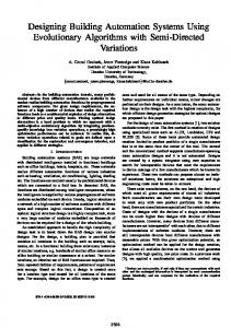
Type III: DG capable of injecting both real and reactive power, e.g. synchronous machines. Type IV: DG capable of injecting real but consuming reactive power, e.g. induction generators used in the wind farms. In past various approaches have been applied to penetrate the DG location and sizing in distribution network. These approaches place DG in the system with the aim of minimizing the power losses. Surprisingly all these approaches are addressed with particular loading conditions, however in real time application these load levels are dynamic and may be the approach gives erroneous results when subjected to a particular operating condition. Various approaches like Ant Colony Optimization, Evolutionary Algorithm (EA) and Particle Swarm Optimization (PSO) [2]-[5]. In[4] a new improved harmony search algorithm to address the placement of DGs in distribution networks. The results are compared with Non dominated Sorting Genetic Algorithm (NSGA) and Particle Swarm Optimization (PSO) .In [7] placement of renewable sources namely wind and solar was done with the help of evolutionary programming. Authors reported two operation strategies, namely “turning off wind turbine generator” and “clipping wind turbine generator output”. These strategies were adopted to restrict the wind power dispatch to a specified fraction of system load for system stability consideration. Further the approaches like Prime Dual Interior Point method [8], mixed integer nonlinear programming [9],[10], evolutionary programming (EP) technique [11], analytical approach [12]–[15], trade-off method [16], Hereford Ranch algorithm [17], linear programming technique [18], genetic algorithm(GA) technique [19], heuristic approaches [20], Classical Second Order method [21], Tabu Search approach [22],and Decision Theory approach [23] have been employed to solve the Dg placement problem in Distribution Networks. 2. PARTICLE SWARM OPTIMIZATION Particle swarm optimization is a stochastic population based evolutionary algorithm for problem solving. Particle swarm optimization is a stochastic, population-based evolutionary computer algorithm for problem solving. It is a kind of swarm intelligence that is based on social-psychological principles and provides insights into social behavior, as well as contributing to engineering applications. The particle swarm optimization algorithm was first described in 1995 by JAMES KENNEDY and RUSSELL C.EBERHART [24]. In a PSO system, particles fly around in a multidimensional search space. During flight, each particle adjusts its position according to its own experience (This value is called Pbest), and according to the experience of a neighboring particle (This value is called Gbest), makes use of the best position encountered by itself and its neighbor fig.1. X ik +1 Vi k
Vi k +1
Gbesti
Vi Gbest X ik
Vi Pbest
Pbesti
Fig.1 : Basic concept of PSO 176
J. Automation & Systems Engineering 8-3 (2014): 175-186
Where
Vi k is current velocity of particle i at iteration k. Vi k +1 is modified velocity of particle i. X ik is current position of particle i at iteration k . X ik +1 is modified position of particle i. Vi Pbest is velocity based on Pbest . Vi Gbest is velocity based on Gbest . This modification can be represented by concept of velocity. Velocity of each agent can be modified by following equation:
Vi k +1 = wVi k + c1 rand * ( pbest i − X ik ) + c 2 rand * ( gbest i − X ik ) Using above equation, a certain velocity, which gradually gets close to pbest and gbest can be calculated. The current position (searching point in the solution space) can be modified by following equation:
X ik +1 = X ik + Vi k +1 This is expected to move the swarm toward the best solutions. Such methods are commonly known as heuristics as they make few or no assumptions about the problem being optimized and can search very large spaces of candidate solutions.PSO can therefore also be used on optimization problems that are partially irregular, noisy, change over time, etc. 3. Radial Basis Function Neural Network The RBFNN is a feed forward neural network consisting of three layers namely, an input layer which feeds the values to each of the neurons in the hidden layer, a hidden function which consists of neurons with radial basis activation function and an output layer which contains neurons with linear activation function. The learning process for RBF neural networks is composed of initiating centers and widths for RBF units and computing weights for connectors of these units. Based on different applications of RBFNN, in the literature many learning strategies have been applied for changing the parameters of RBFNN during the training process. The conventional learning algorithm applied for real time application cannot satisfy the desired speed and performance in the training process. Hence, the optimum steepest descent learning algorithm is applied to improve the RBFNN training process with fewer epochs so as to make it faster and more accurate .A generic topology of RBFNN with k input and m hidden neurons is shown in Fig.2. For the training of the RBFNN and considering a k dimensional input vector, X, the computed scaler values can be expressed as,
Y = f (X ) = W 0 +
m
∑ W Φ(D i
i
)
(1)
i =1
Where ܹ is the bais, ܹ is the weight parameter,݉ is the number of neurons in the hidden layer and (Di) is the RBF. There are many basis functional choices possible for the RBF like spline, multi-quadratic, and Gaussian functions but the most widely used one is the Gaussian function. The
177
S. Gupta et al.: A Radial Basis Function NN based Optimal Placement of DG in Distribution Networks
Gaussian RBFNN is found not only suitable in generalizing a global mapping but also in refining local features without altering the already learned mapping. In this study, the Gaussian function is used as the RBF and it is given by − D i2 (2) φ ( D i ) = exp 2 σ
Here σ is the radius of the cluster represented by the center node (Spread) and usually called ݐ݀݅ݓℎ, ݅ܦ, is the distance between the input vector and X and all data centers. The Euclidean norm is normally used to calculate the distance, ܦ which is given by k
Di =
∑(X
j
(3)
− f ji ) 2
j =1
Where ݂ is the cluster center for any of the given neurons in the hidden layer. Input X1
Weights
Radical basis function
Linear weights W0
f1
W1
+ Input X2
O utput Y
W2
f2
W m
fm Hidde n Layer
Input XK
Input Laye r
Fig. 2 : A Generic architecture of RBFNN
178
O utput Layer
J. Automation & Systems Engineering 8-3 (2014): 175-186
Start
input the syste m parameters
establishme nt of data set
carry out the load flow analysis to calculate loss for base case
Generate the initial population of particles
set iteration count k=0
check if all constraints satisfy
No
set infeasible data to base case
Y es
evaluate each particle initialize pbest as current position for all particles assign gbest as best among pbest
update weight velocity & position of all particles
update pbest if new position is better than pbest
update gbest if new position of gbest is better than previous gbest
k=k+1
Y es
if k