J5.1 VALIDATION OF CFD SIMULATION OF TURBULENT AIR FLOW OVER A REGULAR ARRAY OF CUBES AGAINST WIND TUNNEL DATA AND A 3D ANALYSIS OF THE FLOW *
Jose Luis Santiago , Alberto Martilli and Fernando Martin CIEMAT (Center for Research on Energy, Environment and Technology). Madrid, Spain.
1. INTRODUCTION Air pollution in urban canopy represents an important environmental problem and the study of pollutant dispersion in cities is not easy. The interaction between atmospheric flow and urban obstacles such as buildings generates a complex flow in streets affecting pollutant dispersion. Wind tunnel experiment with different geometries (e.g., Brown et al., 2001; Meroney et al., 1996) have been carried out. Other useful tools to study building-air flow interactions are Computational Fluid Dynamics models (CFD). CFD model simulations play an important role in the understanding of microscale flow features and their results can be useful for urban parameterizations in high resolution mesoscale models. Thus, a large number of numerical investigations have been also made such as Baik and Kim (1999), Chan et al. (2003), Lien and Yee (2004), Santiago and Martin (2005), Sini et al. (1996), etc. In this contribution, air flow over a regular array of cubes is simulated by a CFD. Simulation is based on Reynolds Averaged Navier-Stokes equations (RANS) using standard k -ε turbulent closure. CFD results are validated against wind tunnel measurements. Some statistical parameters (correlation coefficients, fractional BIAS and normalised mean square error) are computed and a validation test (Schlünzen et al., 2004) is applied. Comparison shows that the complex flow structure over building array obtained by CFD is in good agreement with wind tunnel data. In addition, a three-dimensional analysis of the air flow structure inside street canyons is carried out. 2. SET UP The array used has 7 (streamwise direction) x 11 (spanwise direction) cubes. Cube edge length (H = 0.15 m) and spacing between cubes in both directions are the same and equal to 0.15 m. X-, Y-, Z-axis are located in streamwise, spanwise and vertical direction, respectively, and the origin of coordinate system is situated at *
Corresponding author address: Jose Luis Santiago, CIEMAT, Dept. of Environment, Av. Complutense 22, 28040, Madrid, Spain; email:
[email protected]
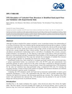
ground in the middle of upwind face of the first cube in the streamwise direction (see Figure 1). Wind tunnel experiment is carried out by Brown et al. (2001). In this study, numerical simulation is made by a CFD (FLUENT). Thus, computed results are compared with wind tunnel data and airflow structures are analysed. Numerical domain are shown in Figure 1 where only one row of buildings in X-direction with symmetric conditions at Y/ H = -1 and 1 is simulated. This configuration is equivalent to simulating an infinite array of cubes in spanwise direction (see Figure 1), ensuring a less CPU time spent.
Figure 1. The a) side view and b) top view of the numerical domain and grid system. Numerical domain stretches from X/ H = -5 to 28 in the streamwise direction, from Y/ H = -1 to 1 in the spanwise direction and from Z/H = 0 to 8 in the vertical direction. A 202 x 44 x 40 irregular Cartesian grid is used which have more resolution inside canyons and close to cubes, and decreases farther from them (see Figure 1). Wind tunnel data are used to set up inflow velocity and turbulent kinetic energy. 3. MODEL DESCRIPTION Airflow over cubic array is simulated by FLUENT model using steady Reynolds NavierStokes (RANS) equations with the k -ε turbulence closure scheme. The governing equations are solved in a collocated grid system using finite volume method. Pressure-velocity coupling is solved by means of SIMPLE (Patankar, 1980)
algorithm and the QUICK scheme (Leonard, 1979) is used as advection-differencing scheme. 4. RESULTS The evaluation against wind tunnel data of the performance of the FLUENT code simulating airflow over the array is one of the objective of this work. In addition, the other aim is to study airflow behavior over the array. 4.1 Evaluation Procedure Simulation results (mean streamwise velocity, U, mean vertical velocity, W and turbulent kinetic energy, TKE) are compared with wind tunnel data in several locations at Y/H = 0 shown in Figure 2. A statistical analysis is made by means of variables such as normalised mean square error (NMSE) (eq. 1), fractional BIAS (FB) (eq. 2) and correlation coefficient (R) (eq. 3), and a validation test (Schlünzen et al., 2004) (eq. 4). n
NMSE =
∑ (O
i
− Pi ) 2
i =1 n
(1)
∑ (Oi ⋅ Pi ) i =1
FB =
O −P 0 .5 ⋅ (O + P )
∑ [(O n
R=
i =1
i
1 if
]
− O )( Pi − P )
n (O i − O ) 2 ∑ i =1 n N 1 q= = ∑Ni n n i =1 Ni =
(2)
1/ 2
n (Pi − P ) 2 ∑ i =1
(3)
1/ 2
with
Pi − Oi ≤ RD or Pi − Oi ≤ AD Oi 0 else
NMSE FB R U 0.009 -0.082 0.997 W 0.396 0.396 0.926 TKE 0.159 0.122 0.680 Table 1. NMSE, FB and R values for U, W and TKE. Number of Number of Hit Rate Points Hits (q) U 248 235 95% W 248 190 77% TKE 248 201 81% Table 2. Validation hit rate results. In addition, U, W and TKE vertical profiles obtained by numerical simulations and wind tunnel experiments are compared in several locations shown in Figure 2.
(4)
where n is the number of points, the
Oi are the
measurements at each point, and
O is the
measurement mean.
Hit rate validation test (Schlünzen et al., 2004) is applied for U, W and TKE using a relative deviation of RD = 0.25 for all variables -1 and an absolute deviation of AD = 0.15 m s for 2 -2 U and W, and AD = 0.15 m s for TKE. Regarding values of RMS, FB and R shown in Table 1 and results of hit rate validation test shown in Table 2 we conclude: 1) For U excellent comparison results (q = 95% and NMSE = 0.009) with a high R and a general light overestimation. 2) For W good comparison results (q = 77%) (fulfilled test criterion which is q > 66%) and excellent correlation 3) For TKE good comparison results (q = 81% and NMSE = 0.159) but less satisfactory results for correlation as compared with the previous variables. In addition, a light underestimation is observed. In general, the performance of FLUENT comparing with wind tunnel data is considered highly satisfactory.
Pi and P are computed
values at each point and the corresponding mean, respectively (Hanna et al., 1991; Santiago et al., 2005; Wilks, 1995). NMSE is a value of normalised discrepancies between computed and experimental values. FB indicates the existence of over- or under-estimation. Figure 3. U, W and TKE vertical profiles at M and N locations.
Figure 2. Location of profiles compared.
Analysing all profiles, as expected, there is notably good agreement in U comparison, only there are light differences above cube rooftops. Regarding W, the agreement is fairly good but
model overestimates W intensity (inside canyon underestimates negative values and above them overestimates positive values). Considering TKE, simulation results and wind tunnel data has similar shape, but it is underestimated inside the canyons. Other important feature is the similar behavior of U, W, TKE inside canyons and above cube rooftops from the fourth canyon to the end of the array, as example in Figure 3 is th depicted vertical profiles at M location (inside 4 th canyon) and at N location (above the 5 cube rooftop). In general, the performance of FLUENT is in agreement with experimental data and the results can be used to analyse flow structures. 4.2 Wind Flow Pattern (3-D Analysis)
U
W
Complex flow patterns are created inside the cube array and its study is important for example to analyse pollutant dispersion. An interesting zone to study is at the canyon center plane, Y / H = 0 (Figure 4). Here, there are asymmetric vortices inside canyons with a more intense downward motion at the windward wall than the upward motion at the leeward. TKE highest values are located where the flow gradients are high (at the beginning of the array and in the canyon upper downwind corner). It is interesting to note the flow stationary inside canyons seems to be reached, from the fourth canyon to the end similar wind flow pattern are created. The largest differences are found in the first canyon and in less proportion the last one which are influenced by the edges of the array.
a)
TKE b) U (m s
-1
)
W (m s
-1
)
2
-2
TKE (m s )
c)
d)
Figure 4. U, W and TKE flow patterns and the vector map inside the fourth canyon at Y /H=0.
Figure 5. Vector map and W contours zoomed in the fourth canyon at: a) Z / H = 0.25; b) Z / H = 0.5; c) Z / H = 0.75; d) Z / H = 1. Color scale is the same as Figure 4 for W.
To complete flow analysis, it is studied in several horizontal slices at Z / H = 0.25, 0.5, 0.75 and 1 (zoomed in the fourth canyon, figure 5). At upper region (Z / H = 1) there is a shear zone due to the flow separation in two part, one enters into the canyons by windward face and the other is deflected over the cubes. At lower heights (Z / H = 0.75 and 0.5) the flow enters the canyon laterally from the street. However, close to the ground (Z / H = 0.25), the downward motion at canyon windward face generates divergent horizontal flow, airflow out of the canyon laterally from the street. Near downwind face of street canyons the flow is downward and outward at the lower zone, and downward and inward at the upper region. 5. CONCLUSIONS In this contribution, the airflow inside a 3-D cubic array is simulated by a CFD model and computed results are analysed and compared with wind tunnel data. The main conclusions can be summarized: CFD simulation satisfactorily reproduces the flow structure observed in the wind tunnel. Complex 3-D patterns are induced inside street canyons. Airflow enters (at Z / H = 0.75 and 0.5) and exits (near the ground) the canyons laterally from the street generating patterns very different from 2-D flow structures. 6. ACKNOWLEDGEMENTS The authors wish to thank CIEMAT for the doctoral fellowship held by Jose Luis Santiago and Dr. Michael J. Brown for providing wind tunnel data. REFERENCES Baik, J-J., and Kim, J-J.: 1999, ‘A numerical study of flow and pollutant dispersion characteristics in urban street canyons’, J. Appl. Meteorol. 38, 1576-1589. Brown, M.J., Lawson, R.E., DeCroix, D.S., and Lee, R. L.:2001, Comparison of centreline velocity measurements obtained around 2D and 3D buildings arrays in a wind tunnel, Report LAUR-01-4138, Los Alamos National Laboratory, Los Alamos. Chan, A.T., Au, W.T.W., So, E.S.P.: 2003, ‘Strategic guidelines for street canyon geometry to achieve sustainable street air quality-part II: multiple canopies and canyons’, Atmos. Environ. 37, 2761-2772.
Hanna, S.R., Strimaitis, D.G., and Chang, J.C.: 1991, Hazard response modelling uncertainty (a quantitative method) Volume II. Evaluation of commonly-used hazardous gas dispersion model, Report F08635-89-C-0136, Sigma Research Corporation, Air Force Engineering and Service Center, Tyndal Air Force Base, Florida. Leonard, B. P.: 1979, ‘A stable and accurate convective modelling procedure based on quadratic upstream interpolation’, Comp. Meth. Appl. Mech. Eng. 19, 59-98. Lien, F-S., and Yee, E.: 2004, ‘Numerical modelling of the turbulence flow developing within and over a 3-D building array, part I: A high-resolution Reynolds-averaged NavierStokes approach’, Boundary-Layer Meteorol. 112, 427-466. Meroney, R.N., Pavegeau, M., Rafailidis, S., and Schatzmann, M.: 1996, ‘Study of line source characteristics for 2-D physical modelling of pollutant dispersion in street canyons’, J. Wind Eng. Indust. Aero. 62, 37-56. Patankar, S.V.: 1980, Numerical Heat Transfer and Fluid Flow, Hemisphere Publishing Corporation, New York. Santiago, J.L., and Martin, F.: 2005, ‘Modelling the air flow in symmetric and asymmetric street canyons’, Int. J. Environ. Pollut. 25, 145-154. Santiago, J.L., Sanz-Andres, A., and Martin, F.: 2005, ‘Experimental and numerical study of a type of windbreaks to reduce dust emissions in st harbours’ in 1 International Conference on Harbours & Air Quality, Genoa, June 15-17, Italy. Schlünzen, K.H., Bächlin, W., Brünger, H., Eichhorn, J., Grawe, D., Schenk, R., and Winkler, C.: 2004, ‘An evaluation guideline for th prognostic microscale wind field models’ in 9 International Conference on Harmonisation within Atmospheric Dispersion Modelling for Regulatory Purposes, Garmisch-Partenkirchen, June 1-4, Germany. Sini, J-F., Anquetin, S. and Mestayer, P.G.: 1996, ‘Pollutant dispersion and thermal effects in urban street canyons’, Atmos. Environ. 30, 2659-2677. Wilks, D. S.: 1995, Statistical Methods in Atmospheric Sciences, Academic Press, San Diego.