Apr 24, 2013 - to the discovery of Macdonald polynomials [Mac95] and Jack .... torus) and (b) an example of its embedding F(Σ) = α, ...... Kevin W. J. Kadell.
arXiv:1301.6531v2 [math.CO] 24 Apr 2013
JACK POLYNOMIALS AND ORIENTABILITY GENERATING SERIES OF MAPS ´ MACIEJ DOŁEGA, ˛ VALENTIN FÉRAY, AND PIOTR SNIADY A BSTRACT. We study Jack characters, which are the coefficients of the power-sum expansion of Jack symmetric functions with a suitable normalization. These quantities have been introduced by Lassalle who formulated some challenging conjectures about them. We conjecture existence of a weight on maps (i.e., graphs drawn on surfaces), allowing to express Jack characters as weighted sums of some simple functions indexed by maps. We provide a candidate for this weight which gives a positive answer to our conjecture in some, but unfortunately not all, cases. This candidate weight measures somehow the non-orientability of a given map.
1. I NTRODUCTION 1.1. Jack polynomials and Macdonald polynomials. In a seminal paper [Jac71], Jack introduced a family of symmetric polynomials — which are (α) now known as Jack polynomials Jπ — indexed by an additional deformation parameter α. From the contemporary viewpoint probably the main motivation for studying Jack polynomials comes from the fact that they are a special case of the celebrated Macdonald polynomials which “have found applications in special function theory, representation theory, algebraic geometry, group theory, statistics and quantum mechanics” [GR05]. Indeed, some surprising features of Jack polynomials [Sta89] have led in the past to the discovery of Macdonald polynomials [Mac95] and Jack polynomials have been regarded as a relatively easy case [LV95] which later allowed understanding of the more difficult case of Macdonald polynomials [LV97]. A brief overview of Macdonald polynomials (and their relationship to Jack polynomials) is given in [GR05]. Jack polynomials are also interesting on their own, for instance in the context of Selberg integrals [Kad97] and in theoretical physics [FJMM02, BH08]. 2010 Mathematics Subject Classification. Primary 05E05; Secondary 05C10, 05C30, 20C30 . Key words and phrases. Jack polynomials, Jack characters, maps, topological aspects of graph theory. 1
2
´ M. DOŁEGA, ˛ V. FÉRAY, AND P. SNIADY
4 6
6 7
1
5 3 2 4
Figure 1.1. Example of an oriented map. The map is drawn on a torus: the left side of the square should be glued to the right side, as well as bottom to top, as indicated by arrows. 1.2. Jack polynomials, Schur polynomials and zonal polynomials. For some special choices of the deformation parameter α, Jack polynomials coincide (up to some simple normalization constants) with some very established families of symmetric polynomials. In particular, the case α = 1 corresponds to Schur polynomials, α = 2 corresponds to zonal polynomials and α = 21 corresponds to symplectic zonal polynomials; see [Mac95, Chapter 1 and Chapter 7] for more information about these functions. For these special values of the deformation parameter Jack polynomials are particularly nice because they have some additional structures and features (usually related to algebra and representation theory) and for this reason they are much better understood. 1.3. Jack polynomials and maps. Roughly speaking, a map is a graph drawn on a surface, see Figure 1.1. In this article we will investigate the relationship between combinatorics of Jack polynomials and enumeration of maps. In the special cases of Schur polynomials (α = 1) and zonal polynomials (α = 2 and α = 21 ) this relationship is already well-understood. The generic case is much more mysterious and we will be able only to present some conjectures. 1.4. Normalized characters. The irreducible character χλ (π) of the symmetric group is usually considered as a function of the partition π, with the Young diagram λ fixed. It was a brilliant observation of Kerov and Olshanski [KO94] that for several problems in asymptotic representation theory
JACK POLYNOMIALS AND ORIENTABILITY GENERATING SERIES OF MAPS
3
it is convenient to do the opposite: keep the partition π fixed and let the Young diagram λ vary. It should be stressed that the Young diagram λ is arbitrary, in particular there are no restrictions on the number of boxes of λ. In this way it is possible to study the structure of the series of the symmetric groups S1 ⊂ S2 ⊂ · · · and their representations in a uniform way. This concept is sometimes referred to as dual approach to the characters of the symmetric groups. In order for this idea to be successful one has to replace the usual characters χλ (π) by, so called, normalized characters Chπ (λ). Namely, for a partition π of size k and a Young diagram λ with n boxes we define ( λ (π) (n)k χχλ (id) if k ≤ n, (1.1) Chπ (λ) = 0 otherwise, where (n)k := n(n − 1) · · · (n − i + 1) {z } | k factors
denotes the falling factorial. This choice of normalization is justified by the fact that so defined characters Chπ belong to the algebra of polynomial functions on the set of Young diagrams [KO94], which in the last two decades turned out to be essential for several asymptotic and enumerative problems of the representation the´ ory of the symmetric groups [Bia98, IO02, DFS10]. 1.5. Jack characters. Lassalle [Las08a, Las09] initiated investigation of a kind of dual approach to Jack polynomials. Roughly speaking, it is the investigation (as a function of λ, with π being fixed) of the coefficient standing (α) at pπ,1,1,... in the expansion of Jack symmetric polynomial Jλ in the basis of power-sum symmetric functions. The motivation for studying such quantities comes from the observation that in the important special case of Schur polynomials (α = 1) one recovers in this way the normalized characters Ch(1) π = Chπ given by (1.1) which already proved to have a rich and fascinating structure. The cases of zonal polynomials, symplectic polynomials and general Jack polynomials ´ give rise to some new quantities for which in [FS11b] we coined the names (2) zonal characters Chπ , symplectic zonal characters Ch(1/2) and general π (α) Jack characters Chπ . Another motivation for studying Jack characters Ch(α) π comes from the observation that they form a linear basis of the algebra of α-polynomial functions on the set of Young diagrams (which is a simple deformation of the algebra of polynomial functions mentioned above). This fact is far from being trivial and was established by Lassalle [Las08a, Proposition 2].
´ M. DOŁEGA, ˛ V. FÉRAY, AND P. SNIADY
4
2 W 3
V
Σ 5
β
1, 4
α
2, 5
Π
W
V Π
4 1
1
3
Σ
2
a (a)
b
c (b)
Figure 1.2. (a) Example of a bipartite graph (drawn on the torus) and (b) an example of its embedding F (Σ) = α, F (Π) = β, F (V ) = a, F (W ) = c, F (1) = F (4) = (aβ), F (2) = F (5) = (aα), F (3) = (cα). The columns of the Young diagram were indexed by small Latin letters, the rows by small Greek letters. The main goal of this paper is to understand the combinatorial structure of Jack characters Ch(α) π . In the following we will give more details on this problem. 1.6. Embeddings of bipartite graphs. An embedding F of a bipartite graph G to a Young diagram λ is a function which maps the set V◦ (G) of white vertices of G to the set of columns of λ, which maps the set V• (G) of black vertices of G to the set of rows of λ, and maps the edges of G to boxes of λ, see Figure 1.2. We also require that an embedding preserves the relation of incidence, i.e., a vertex V and an incident edge E should be mapped to a row or column F (V ) which contains the box F (E). We denote by NG (λ) the number of such embeddings of G to λ. Quantities NG (λ) ´ were introduced in our paper [FS11a] and they proved to be very useful for studying various asymptotic and enumerative problems of the representa´ ´ tion theory of symmetric groups [FS11a, DFS10]. 1.7. Stanley formulas. We will recall formulas that express Jack � 1charac (α) ters Chπ in terms of functions NG in the special cases α ∈ 2 , 1, 2 . Formulas of this type are called Stanley formulas after Stanley, who found such a formula for α = 1 as a conjecture [Sta06]. 1.7.1. Stanley formula for α = 1 and oriented maps. Roughly speaking, an oriented map M is defined as a bipartite graph drawn on an oriented
JACK POLYNOMIALS AND ORIENTABILITY GENERATING SERIES OF MAPS
5
surface, see Figure 1.1. Since oriented maps are not in the focus of this article, we do not present all necessary definitions and for details we refer ´ to [FS11a]. ´ It has been observed in [FS11a] that a formula conjectured by Stanley and proved by the second author [Sta06, Fér10] for the normalized characters of the symmetric groups can be expressed as the sum X ℓ(π) (1.2) Ch(1) (λ) = Ch (λ) = (−1) (−1)|V• (M )| NM (λ) π π M
over all oriented bipartite maps M with face-type π. Here and throughout the paper, NM denotes the function N indexed by the underlying graph of map M.
1.7.2. Stanley formula for α = 2, α = 21 and non-oriented maps. Roughly speaking, a non-oriented map is a bipartite graph drawn on a surface. For a precise definition (and definition of face-type) we refer to Section 3.2. ´ In [FS11b] it has been proved that X � 1 �|V• (M )| �√ �|V◦ (M )| (2) ℓ(π) (1.3) Chπ (λ) = (−1) −√ 2 2 M �|π|+ℓ(π)−|V (M )| � 1 NM (λ), · −√ 2 X � √ �|V• (M )| � 1 �|V◦ (M )| √ (1.4) = (−1) − 2 2 M � �|π|+ℓ(π)−|V (M )| 1 · √ NM (λ), 2 where the sums run over all non-oriented maps M with the face-type π. ´ Notations and presentation in [FS11b] are a little bit different, so we ´ make the link between the results above and statements in [FS11b] in Section 5.1. Ch(1/2) (λ) π
ℓ(π)
1.8. The main conjecture. Based on the special cases above, on some theoretical results of this paper and some computer exploration, we formulate the following conjecture: Main Conjecture 1.1. To each map M, one can associate some weight wtM (γ) such that • wtM (γ) is a polynomial with non-negative rational coefficients in γ of degree (at most) d(M) := 2(number of connected components of M ) − χ(M),
´ M. DOŁEGA, ˛ V. FÉRAY, AND P. SNIADY
6
where χ(M) := |V (M)| − |E(M)| + |F (M)|
is the Euler characteristic of M. Moreover, the polynomial wtM (γ) is an even (respectively, odd) polynomial if and only if the Euler characteristic χ(M) is an even number (respectively, an odd number). • for every λ and π, the following formula holds � � X � 1 �|V• (G)| √ �|V◦ (G)| 1−α (α) ℓ(π) √ −√ α Chπ (λ) = (−1) NM (λ), wtM α α M where the sum runs over all non-oriented maps M with the facetype specified by π.
Throughout the paper, we shall denote γ = γ(α) :=
1−α √ . α
We know that Ch(α) π can be written as a linear combination of functions NG over some bipartite graphs G: it is a consequence of the fact that Ch(α) π is an α-shifted symmetric function, see [Las08a, Proposition 2]. However, since functions NG , seen as functions on Young diagrams, are not linearly independent [Fér09, Proposition 2.2.1], this expansion is not unique; therefore our conjecture should be understood as a claim about the existence of a particularly nice expansion of Ch(α) π in terms of functions NG . 1.9. A concrete version of the conjecture. As we have seen above, the case α = 1 (Eq. (1.2)) corresponds to summation over oriented maps, while the cases α = 2 and α = 21 correspond to summation over non-oriented maps (Eqs. (1.3), (1.4)) with some simple coefficients which depend only on general features of the map, such as the number of the vertices. Thus one can expect that the coefficient wtM (γ) should be interpreted as a kind of measure of non-orientability of a given map M. This notion of measure of non-orientability is not very well defined. For example, one could require that for α = 1 the corresponding coefficient wtM (0) is equal to 1 if M is orientable and zero� otherwise; and that for � �1 1 1 α ∈ 2 , 2 and γ(α) = ± √2 the coefficient wtM ± √2 takes some fixed value on all (orientable and non-orientable) maps. In Section 3.8 we will define some quantity monM = monM (γ) which indeed — although in some perverse sense — measures non-orientability of a given map M. Note that monM depends on γ(α) and thus on α but we drop this dependence in the notation. Roughly speaking, monM is defined as follows: we remove edges of the map M one after another in a random order. For each edge which is to be removed we check the type of this edge (for example, an edge may be twisted if, in some sense, it is a part of Möbius
JACK POLYNOMIALS AND ORIENTABILITY GENERATING SERIES OF MAPS
7
band). We multiply the factors corresponding to the types of all edges. The quantity monM is defined as the mean value of this product. This is a rather strange definition. For example, one could complain that this is a weak measure of non-orientability of a map; in particular for α = 1 the corresponding weight monM does not vanish on non-orientable maps. Nevertheless, this weight monM often (but not always!) gives a positive answer to our Main conjecture. We state it precisely as the following conjecture. Conjecture 1.2. For arbitrary Young diagram λ, partition π and α > 0, the value of Jack character is given by (1.5) X � 1 �|V• (G)| √ �|V◦ (G)| (α) ℓ(π) −√ Chπ (λ) = (−1) α monM NM (λ), α M where the summation runs over all non-oriented maps with face-type π.
With extensive computer calculations we were able to check that Conjecture 1.2, in general, not true; the simplest counterexample is π = (9) (see Section 7 for more details). Nevertheless, as we shall present in the following, it seems that this conjecture predicts some properties of Jack characters surprisingly well. We hope that investigation of Conjecture 1.2 might shed some light on the problem and eventually lead to the correct formulation of the solution of Main Conjecture 1.1. For example, the conjecture holds true for the following special cases: λ = (n) which consists of a single part for 1 ≤ n ≤ 8, furthermore for λ = (2, 2), and λ = (3, 2) (the proofs are computer-assisted). Corollary 4.3 shows that the conjecture holds also for any of these partitions augmented by an arbitrary number of parts equal to 1. In a forthcoming paper ´ [CJS13] we will present a human-readable proof that Conjecture 1.2 is true for partitions π = (n) consisting of a single part for 1 ≤ n ≤ 6. In the following (Section 1.11, Section 1.12, Section 1.13.1) we will present some other special cases for which Conjecture 1.2 seems to be true. 1.10. Orientability generating series. We define the orientability generc (α) (λ) as the right hand-side of (1.5): ating series Ch π
c (α) (λ) := (−1)ℓ(π) Ch π
X� M
1 −√ α
�|V• (M )|
√ �|V◦ (M )| α monM NM (λ),
where the sum runs over all non-oriented maps M with the face-type π. With this notation, Conjecture 1.2 may be equivalently reformulated as
´ M. DOŁEGA, ˛ V. FÉRAY, AND P. SNIADY
8
follows: for any partition π the corresponding Jack character and the orientability generating series are equal: c (α) Ch(α) π (λ) = Chπ (λ).
1.11. Rectangular Young diagrams. Investigation of the normalized characters Chπ (λ) in the case when λ = p × q is a rectangular Young diagram was initiated by Stanley [Sta04] who noticed that they have a particularly simple structure; in particular he showed that formula (1.2) holds true in this special case. This line of research was continued by Lassalle [Las08a] who (apart from other results) studied Jack characters Ch(α) π (p × q) on rectangular Young diagrams. In particular, Lassalle found a recurrence relation [Las08a, formula (6.2)] fulfilled by such characters; this recurrence relates values of the characters on a fixed rectangular Young diagram p × q, corresponding to various partitions π. This recurrence relation is essential for the current paper; Conjecture 1.2 was formulated by a careful attempt of reverse-engineer the hidden hypothetical combinatorial structure behind Lassalle’s recurrence. In particular, our measure of non-orientability of maps monM was from the very beginning chosen in such a way that Conjecture 1.2 is true for an arbitrary rectangular Young diagram λ = p×q. We will discuss these issues and prove Conjecture 1.2 for rectangular Young diagrams in Section 4. Extensive computer exploration leads us to believe that Conjecture 1.2 might be true if the Young diagram λ is not far from being rectangular. We state it precisely as follows (the missing notation will be presented in Section 7). Conjecture 1.3. Conjecture 1.2 is true if λ = (p1 , p2 ) × (q1 , q2 ) is a multirectangular Young diagram consisting of (at most) two rectangles. Our computer exploration supports this conjecture. It would imply explicit formulas for quadratic terms of Kerov polynomials for Jack characters (analogous formulas for the linear terms are known to hold true because Conjecture 1.1 holds true for rectangular Young diagrams); for details see ´ [CJS13]. 1.12. Top-twisted part. Conjecture 1.4. The top-twisted parts of the Jack character and the orientability generating series are equal, i.e. for any partition π and any Young diagram λ lim
1
s→∞ s|π|+ℓ(π)
Ch(sα) π (sλ) = lim
1
s→∞ s|π|+ℓ(π)
c (sα) (sλ). Ch π
JACK POLYNOMIALS AND ORIENTABILITY GENERATING SERIES OF MAPS
9
´ For details and the missing notation we refer to [CJS13]. Our computer exploration supports this conjecture. 1.13. Links with other problems. 1.13.1. Lassalle’s conjectures. Looking for some Stanley formula for general Jack characters Ch(α) π has been motivated by two recent conjectures of Lassalle. He conjectured some nice positivity and integrality properties for the coefficients of Ch(α) π expressed, respectively, in terms of multirectangular coordinates [Las08a, Conjecture 1 and Conjecture 2] and free cumulants [Las09, Conjecture 1.1 and Conjecture 1.2]. The positivity part in both conjectures would follow from our Main Conjecture 1.1: for multirectangular coordinates we explain the connection in Section 6, while for free cumu´ lants this would follow from the general machinery developed in [DFS10]. The conjecture of Lassalle involving free cumulants is supported by a ´ huge amount of numerical data [Las08b]. In a forthcoming paper [CJS13], we shall show that the predictions of Conjecture 1.2 coincide with this data for the four highest-degree components. This gives even more evidence towards Conjecture 1.2 (which is, unfortunately, false in general). 1.13.2. The b-Conjecture of Goulden and Jackson. In the current paper we investigate the combinatorics of Jack characters related to maps. The study of analogous connections between Jack polynomials and maps is much older. In particular, Goulden and Jackson [GJ96a] formulated a conjecture (called b-Conjecture) which claims, roughly speaking, that the connection coefficients of Jack polynomials can be explained combinatorially as summation over certain maps with coefficients that should describe nonorientability of a given map. An extensive bibliography to this topic can be found in [LC09]. Although there is no direct link between our problem and the b-Conjecture (we are unable to show, for instance, that one implies the other), both problems seem quite close and we hope that any progress on one of them could give ideas to solve the other. 1.14. Outline of the paper. In Section 2, we define Jack characters. Then, in Section 3, we give formal definitions related to non-oriented maps and define the weight monM . In Section 4 and Section 5, we prove that �Conjecture 1.2 holds respectively for rectangular Young diagrams and α ∈ 21 , 2} . In Section 6, we explain the link between our Main Conjecture and some conjectures of Lassalle. Then finally, in Section 7, we present our numerical exploration and the counterexample.
´ M. DOŁEGA, ˛ V. FÉRAY, AND P. SNIADY
10
2. P RELIMINARIES 2.1. Partitions and Young diagrams. A partition π = (π1 , . . . , πl ) is defined as a weakly decreasing finite sequence of positive integers. If π1 + · · · + πl = n we also say that π is a partition of n and denote it by π ⊢ n. We will use the following notations: |π| := π1 + · · · + πl ; furthermore ℓ(π) := l denotes the number of parts of π and mi (π) := {k : πk = i} denotes the multiplicity of i ≥ 1 in the partition π. When dealing with partitions we will use the shorthand notation 1l := (1, . . . , 1). | {z } l times
Any partition can be alternatively viewed as a Young diagram. For drawing Young diagram we use the French convention. The conjugacy classes of the symmetric group Sn are in the one-to-one correspondence with partitions of n. Thus any partition π ⊢ n can be also viewed as some (arbitrarily chosen) permutation π ∈ Sn with the corresponding cycle decomposition. This identification between partitions and permutations allows us to define characters such as Tr ρ(π), Ch(α) π for π being either a permutation or a partition. 2.2. Jack characters. Jack characters were introduced by Lassalle [Las08a, Las09]; since we use a different normalization the following presentation is based on our previous work [DF12]. As there are several of them, we have to fix a normalization for Jack polynomials. In our context, the best is to use the functions denoted by J in the book of Macdonald [Mac95, Section VI, Eq. (10.22)]. We expand Jack polynomial in the basis of power-sum symmetric functions: X (α) Jλ = θρ(α) (λ) pρ ; ρ: |ρ|=|λ|
then we define (2.1)
Ch(α) π (λ)
=α
−
|π|−ℓ(π) 2
� � |λ| − |π| + m1 (π) (α) zπ θπ∪1|λ|−|π| (λ), m1 (π)
where zπ = π1 π2 · · · m1 (π)! m2 (π)! · · · .
These quantities Ch(α) π are called Jack characters. It turns out that for α = 1 we recover the usual normalized characters (1.1) of the symmetric groups.
JACK POLYNOMIALS AND ORIENTABILITY GENERATING SERIES OF MAPS
11
2.3. Relationship to Lassalle’s normalization. For reader’s convenience we provide below the relationship between quantities used by Lassalle (in boldface) and the ones used by us: � � |λ| − |π| + m1 (π) λ λ zπ θπ∪1 ϑπ∪1n−|π| (α) = |λ|−|π| (α), m1 (π) (2.2)
− Ch(α) π (λ) = α
|π|−ℓ(π) 2
ϑλπ∪1n−|π| (α).
Our convention has the advantage of being compatible with the symmetry (α, λ) ↔ (α−1 , λ′ ), where λ′ is the transpose diagram of λ [Mac95, Section 1.1]. Namely, |π|−ℓ(π) Ch(α) Ch(1/α) (λ′ ). π (λ) = (−1) π
(2.3) 3. T HE
MEASURE OF NON - ORIENTABILITY OF MAPS
3.1. Pairings and polygons. A set-partition of a set S is a set {I1 , · · · , Ir } of pairwise disjoint non-empty subsets whose union is S. A pairing (or, alternatively, pair-partition) of S is a partition into pairs. If s is an element of S and P is a pairing of S, the partner of s in P is defined as the unique element t ∈ S such that {s, t} is a pair of P . For instance, for any integer n ≥ 1, � P = {1, 2}, {3, 4}, . . . , {2n − 1, 2n}
is a pairing of [2n] (we use the standard notation [n] := {1, · · · , n}). Note that the existence of a pairing of S clearly implies that |S| is even. Let us consider now two pairings B, W of the same set S consisting of 2n elements. We consider the following bipartite edge-labeled graph L(B, W): • it has n black vertices indexed by the two-element sets of B and n white vertices indexed by the two-element sets of W; • its edges are labeled with the elements of S. The extremities of the edge labeled i are the pairs of B and W containing i. Note that each vertex has degree 2 and each edge has one white and one black extremity. Besides, if we erase the indices of the vertices, it is easy to recover them from the labels of the edges (the index of a vertex is the set of the two labels of the edges leaving this vertex). Thus, we forget the indices of the vertices and view L(B, W) as an edge-labeled graph. As every vertex has degree 2, the graph L(B, W) is a collection of polygons. Moreover, because of the proper bicoloration of the vertices, all polygons have even length. Let 2ℓ1 ≥ 2ℓ2 ≥ · · · be the ordered lengths of these polygons. The partition (ℓ1 , ℓ2 , . . . ) is called the type of L(B, W) or the type of the couple (B, W). Special role will be played by polygons having exactly 2 edges. Such a polygon will be referred to as bigon.
´ M. DOŁEGA, ˛ V. FÉRAY, AND P. SNIADY
12
3 4
2
5
1
6
10 7
B
A
C
D
9 8
Figure 3.1. Polygons obtained from a couple of pairings from Example 3.1. Example 3.1. For partitions � B = {1, 2}, {3, 4}, {5, 6}, {7, 8}, {9, 10}, {A, B}, {C, D} , � W = {2, 3}, {4, 5}, {6, 7}, {8, 9}, {10, 1}, {B, C}, {D, A} the corresponding polygons L(B, W) are shown in Figure 3.1.
Let s1 and s2 be two elements of S that belong to the same polygon of L(P1 , P2 ). Fix an arbitrary orientation of this polygon. Then, one can consider the number of elements of S between s1 in s2 in the polygon. We say that s1 and s2 are in an even (respectively, odd) position if this number is even (respectively, odd). As all polygons have even size, this definition does not depend on the choice of the orientation. 3.2. Non-oriented maps. The central combinatorial object in this paper is the following. Definition 3.2. A map is a triplet (B, W, E) of pairings of the same set S. The terminology comes from the fact that it is possible to represent such a triplet of pair-partitions as a bipartite graph embedded in a non-oriented (and possibly non-connected) surface. Let us explain how this works. First, one can consider the union of polygons L(B, W) defined in Section 3.1. The edges of these polygons, that is the elements of the set S are called edge-sides. We consider the union of the interiors of these polygons as a (possibly disconnected) surface with a boundary. If we consider two edge-sides, we can glue them: that means that we identify their white extremities, their black extremities and the edge-side themselves.
JACK POLYNOMIALS AND ORIENTABILITY GENERATING SERIES OF MAPS
13
6 2
C
10
5
D
B
7
A 1
3 8
4 9
10 2
Figure 3.2. Example of a non-oriented map drawn on the projective plane. The left side of the square should be glued with a twist to the right side, as well as bottom to top (also with a twist), as indicated by arrows. This map has been obtained by gluing the edge-sides of the polygon of Figure 3.1 according to the pair-partition give by Eq. (3.1). For any pair in the pairing E, we glue the two corresponding edge-sides. Doing that, we obtain a (possibly disconnected, possibly non-orientable) surface Σ without boundary. After the gluing, the polygons form a bipartite graph G embedded in the surface. For instance, with the pairings B and W from Example 3.1 and � (3.1) E = {1, 3}, {2, 10}, {4, 9}, {5, D}, {6, C}, {7, B}, {8, A} ,
we get the graph from Figure 3.2 embedded in the projective plane. In general, the graph G has as many connected components as the surface Σ. Besides, Σ \ G corresponds to the interiors of the collection of polygons we are starting from. In particular, each connected component of Σ \ G is homeomorphic to an open disc. These connected components are called faces. This makes the link with the more usual definition of maps: usually, a (non-oriented, bipartite) map is defined as a (bipartite) connected graph G embedded in a (non-oriented) surface Σ in such a way that each connected component of Σ \ G is homeomorphic to an open disc. It should be stressed that with our definition — contrary to the traditional approach — we do not require the map to be connected. Definition 3.3. Let M = (B, W, E) be a map.
14
´ M. DOŁEGA, ˛ V. FÉRAY, AND P. SNIADY
• Elements of B (respectively, W) are called black (respectively, white) corners. • Elements of E are called edges; we use the notation E(M) for the set of edges of a map (that is the third element of the triplet defining the map). • The polygons L(B, W) corresponding to the couple of pairings (B, W) are called faces; the set of faces will be denoted F (M). The facetype of the map is the type of the couple (B, W), as defined in Section 3.1. • The polygons L(B, E) (respectively, L(W, E)) of the couple of pairings (B, E) (respectively, (W, E)) are called black vertices (respectively, white vertices); their set is denoted V• (M) (respectively, V◦ (M)). • A leaf of a map M is a vertex of M of degree 1, that is a bigon of L(B, E) or L(W, E). In other terms, a leaf is a pair of edge-sides which belongs to both E and B or which belongs to both E and W. • The connected components of a map M correspond to the connected components of the graph G constructed above. Formally, they are the equivalence classes of the transitive closure of the relation: x ∼ y if x is the partner of y in E, B or W.
Note that our maps have labeled edge-sides and each element of S is used exactly once as a label. The pairing B (respectively, W) indicates which edge-sides share the same corner around a black (respectively, white) vertex. This explains the names of these pairings. This encoding of (non-oriented) maps by triplets of pairings is of course not new. It can for instance be found in [GJ96b]; the presentation in that paper is nevertheless a bit different as the authors consider there connected monochromatic maps. Summation over maps with a specified face-type (such as in (1.3) and (1.4)) should be understood as follows: we fix a couple of pairings (B, W) of type π and consider all pairings E of the same ground set; we sum over the resulting collection of maps (B, W, E). The set of maps with a specified face-type should be understood in an analogous way. 3.3. Three kinds of edges. Let a map M with some selected edge E = {s1 , s2 } be given. We distinguish three cases (a schematic description and an example of each case are given in Figures 3.3 and 3.4): • Both edge-sides s1 and s2 belong to the same face F and are in an even position (see definition at the end of Section 3.1) Graphically, this means that if we travel along the boundary of the face F then we visit the edge E twice and the directions in which we travel twice along the edge E are opposite, see Figure 3.4a.
JACK POLYNOMIALS AND ORIENTABILITY GENERATING SERIES OF MAPS
15
6 C
2 10
5 D
1
B 7 A 8
3 4 9
10 2
Figure 3.3. The non-oriented map from Figure 3.2. On the boundary of each face some arbitrary orientation was chosen, as indicated by arrows. Edge {4, 9} is an example of a straight edge, edge {1, 3} is an example of a twisted edge, edge {6, C} is an example of an interface edge.
(a)
(b)
(c)
Figure 3.4. Three possible kinds of edges in a map (see Figure 3.3): (a) straight edge: both edge-sides of the edge belong to the same face and have opposite orientations, (b) twisted edge: both edge-sides of the edge belong to the same face and have the same orientation, (c) interface edge: the edge-sides of the edge belong to two different faces; their orientations are not important. In all three cases the colors of the vertices are not important. In this case the edge E is called straight and we associate to it the weight 1. • Both edge-sides s1 and s2 belong to the same face F and are in an odd position. Graphically, this means that if we travel along the boundary of the face F , we visit the edge E twice and the directions in which we travel twice along the edge E are the same, see Figure 3.4b.
16
´ M. DOŁEGA, ˛ V. FÉRAY, AND P. SNIADY
In this case the edge E is called twisted and we associate to it the √ . weight γ := 1−α α • Edge-sides s1 and s2 belong to different faces of the map, see Figure 3.4c. In this case the edge E is called interface and we associate to it the weight 12 . The weight given by the above convention will be denoted monM,E . Lemma 3.4. If at least one extremity of an edge is a leaf, then this edge is straight. The proof is a simple exercise. 3.4. Removal of edges. Let P be a pairing of a set S and s1 , s2 be two distinct elements of S. We define a pairing P{s1 ,s2 } of the set S \ {s1 , s2 } as follows: � • if {s1 , s2 } is a pair of P , then P{s1 ,s2 } := P \ {s1 , s2 } . • otherwise, consider the partners t1 and t2 of s1 and s2 . Elements s1 , s2 , t1 , t2 are distinct. We define � � P{s1 ,s2 } := P \ {s1 , t1 }, {s2 , t2 } ∪ {t1 , t2 }. In other words, we remove the pairs containing s1 or s2 and we match together the unmatched pair of elements of S \ {s1 , s2 }.
Lemma 3.5. Let P be a pairing of a set S and s1 , s2 , s3 , s4 be four distinct elements of S. Then � � P{s1 ,s2 } {s3 ,s4 } = P{s3 ,s4 } {s1 ,s2 } . Proof. Easy case by case analysis.
�
Let M = (B, W, E) be a map and E be an edge of M. Then we define M \ {E} (or M \ E) as the triplet (BE , WE , EE ). The lemma above states that, for any two edges E1 , E2 in a map M, one has � � M \ {E1 } \ {E2 } = M \ {E2 } \ {E1 },
which allows to define the map M \ {E1 , · · · , Ei } for an arbitrary subset {E1 , · · · , Ei } ⊆ E(M). Graphically, this corresponds to erasing the edge E in the map M. If one extremity (or both extremities) of this edge is a leaf (are leaves), we also remove it (them). Beware that removal of an edge might change the topology of the surface on which the map is drawn. The following lemma is immediate to prove.
JACK POLYNOMIALS AND ORIENTABILITY GENERATING SERIES OF MAPS
2j edges tW 1
17
2j edges tB 2
s1
s2
tB 1
tB 1
tB 2
tW 1
tW 2
removal of a straight edge
tW 2
2i edges
2i edges
Figure 3.5. Result on faces of a straight edge removal. Lemma 3.6. Let P and P ′ be two pairings of the same base set and let E be a pair in P . Suppose that the couple (P, P ′) has type π and that E lies in a polygon of size r (in particular, r is a part of π). Then, the type of the couple (PE , PE′ ) is obtained from π by replacing a part equal to r by a part equal to r − 1. 3.5. Effect of edge removal on faces. Let us look at the faces of the map M \ {E}, that is the polygons associated to (BE , WE ). 3.5.1. Straight edge removal. Suppose E is a straight edge of M. By definition it means that the two edge-sides s1 , s2 of E belong to the same face F of M. Besides, we know that, if we fix an orientation of F there is an even number, let us say 2i, of the edge-sides between s1 and s2 in F . With the other orientation, there would also be an even number, let us say 2j, of the edge-sides between s1 and s2 in F . This means that the face F has size 2i + 2j + 2 (we call size of a face the number of edges in the corresponding polygon; in particular, it is always an even number). When we remove the edge E, the face F is split into two faces F1 and F2 of respective sizes 2i and 2j (in the degenerate case where i or j is equal to 0, the corresponding face does not exist). This can be easily seen graphically, see Figure 3.5 (here tB1 is the partner of s1 in B, etc.). The other faces are not modified. 3.5.2. Twisted edge removal. Suppose E is a twisted edge of M. By definition it means that the two edge-sides s1 , s2 of E belong to the same face F of M and are in odd position. Let us denote 2r the size of the face F . Then after removal of edge E, the face F is replaced by a face of size 2(r − 1); see Figure 3.6. The other faces are not modified.
´ M. DOŁEGA, ˛ V. FÉRAY, AND P. SNIADY
18
tW 1
tB 2
s2
s1
tB 1
tW 1
tB 2
tW 2
tB 1
removal of a twisted edge
tW 2
2(r − 1) edges in total
2r edges in total
Figure 3.6. Result on faces of a twisted edge removal. 2r edges
tW 1
tB 1 s1 s2
2s edges
tB 2
tW 2
tB 1
removal of an interface edge tB 2
tW 2
tW 1
2(r + s − 1) edges in total
Figure 3.7. Result on faces of an interface edge removal. 3.5.3. Interface edge removal. Suppose E is an interface edge of M. By definition, it means that the two edge-sides s1 , s2 of E belong to different faces F1 and F2 of M. Let us denote 2r and 2s the sizes of faces F1 and F2 . Then after removal of edge E, faces F1 and F2 are replaced by a new face of size 2(r + s − 1); see Figure 3.7. Other faces are not modified. 3.6. Bridges. From the case analysis from Section 3.5 one obtains a result on bridges. Definition 3.7. An edge E of a map M is a bridge if • either at least one of its extremity is a leaf; • or its extremities lie in different connected components of M \ {E}. If E has an extremity of degree 1 (that is, a leaf ), this vertex is not a vertex of M \ {E} anymore, so the second point does not make sense.
JACK POLYNOMIALS AND ORIENTABILITY GENERATING SERIES OF MAPS
19
Lemma 3.8. A bridge is always a straight edge. Proof. Consider a bridge E. If one extremity of E is a leaf, apply Lemma 3.4. Otherwise, the extremities of E lie in different connected components of M \ {E}. But, the case analysis above shows that after removal of a twisted or interface edge, the extremities of this edge lie in the same face and hence in the same connected component of M \ {E}. So E must be straight. � 3.7. Weight associated to a map with a history. Let M be a map and let some linear order ≺ on the edges be given. This linear order will be called history. Let E1 , . . . , En be the sequence of edges of M, listed according to the linear order ≺. We set Mi = M \ {E1 , . . . , Ei } and define Y (3.2) monM,≺ := monMi ,Ei+1 0≤i≤n−1
(we recall that monM,E appearing on the right-hand side was defined in Section 3.3). This quantity monM,≺ can be interpreted as follows: from the map M we remove (one by one) all the edges, in the order specified by the history. For each edge which is about to be removed we consider its weight relative to the current map. Please note that the type of a given edge (i.e., straight versus twisted versus interface) might change in the process of removing edges and the weight monM,≺ usually depends on the choice of the history ≺. 3.8. Measure of non-orientability of a map. Let M be a map with n edges. We define 1 X monM =:= monM,≺ . n! ≺
This quantity can be interpreted as the mean value of the weight associated to the map M equipped with a randomly selected history (with all histories having equal probability). This is the central quantity for the current paper, we call it the measure of non-orientability of the map M. Example 3.9. We consider the map M depicted in Figure 3.8. For calculations involving removal of edges it is more convenient to represent this map as a ribbon graph, see Figure 3.9. For the history EA ≺ EB ≺ EC the corresponding weight is equal to monM,≺ = 1 · 21 · 1 while for the history EB ≺ EA ≺ EC the corresponding weight is equal to monM,≺ = γ · γ · 1. The other histories are analogous to these two cases; finally monM =
2 × 1 · 21 · 1 + 4 × γ · γ · 1 . 6
20
´ M. DOŁEGA, ˛ V. FÉRAY, AND P. SNIADY
EA
EC EB
EC
EA
Figure 3.8. The map M considered in Example 3.9. This map is drawn on Klein bottle: the left-hand side of the square should be glued to the right-hand one (without a twist) and the top side should be glued to the bottom one (with a twist), as indicated by the arrows. For simplicity the labels of the edge-sides were removed and each edge carries only one label.
EA
EB
EC
Figure 3.9. The map from Figure 3.8 drawn as a ribbon graph, i.e., each vertex is represented as a small disc, each edge is represented by a thin ribbon connecting two discs.
JACK POLYNOMIALS AND ORIENTABILITY GENERATING SERIES OF MAPS
21
Lemma 3.10. Let M be a map. Then monM is a polynomial in variable γ of degree (at most) d(M) := 2(number of connected components of M ) − χ(M), where χ(M) := |V (M)| − |E(M)| + |F (M)|
is the Euler characteristic of M. The polynomial monM (γ) is an even (respectively, odd) polynomial if and only if the Euler characteristic χ(M) is an even number (respectively, an odd number). Proof. We claim that for an arbitrary map M and its edge E: (A) monM,E is a polynomial in γ of degree (at most) d(M) − d(M \ E), (B) monM,E is an even (respectively, odd) polynomial if and only if d(M) − d(M \ E) is an even number (respectively, an odd number). Indeed, this statement follows by a careful investigation of each of the three cases considered in Section 3.3 (cases when at least one of the endpoints of E has degree 1 must be considered separately). We present the details in the following. • Assume that both extremities of E are leaves. Then E is straight by Lemma 3.4, so monM,E = 1. But M\{E} has two vertices less, one edge less, one face less and one connected component less than M. So d(M \ {E}) = d(M) and the claim holds in this case. • Assume that exactly one extremity of E is a leaf. Then E is straight by Lemma 3.4, so monM,E = 1. But M\{E} has one vertex less, one edge less, and the same number of faces and connected components than M. So d(M \ {E}) = d(M) and claim holds in this case. • Assume that E is straight, but none of its extremities is a leaf. Recall that monM,E = 1 in this case. But M\{E} has one edge less and one face more (see Section 3.5.1) than M. The number of vertices is unchanged, while the number of connected components can be constant or increase by 1. In the first case, d(M \ {E}) = d(M) − 2 and in the second d(M \ {E}) = d(M). In both cases our claim holds. • Assume that E is twisted. In this case, monM,E = γ. According to Lemma 3.8, the numbers of connected components of M and M \ {E} are the same. The number of faces is not changed either (see Section 3.5.2). The number of edges decreases by 1 and the number of vertices is constant. Thus d(M \ {E}) = d(M) − 1, and our claim holds in this case.
´ M. DOŁEGA, ˛ V. FÉRAY, AND P. SNIADY
22
• Assume that E is an interface edge. In this case, monM,E = 1 . According to Lemma 3.8, the numbers of connected components of M and M \ {E} are the same. The number of faces decreases by 1 (see Section 3.5.3). The number of edges also decreases by 1, while the number of vertices remains the same. Thus d(M \{E}) = d(M), and our claim holds in this case. We apply claims (A) and (B) to each factor on the right-hand side of (3.2); by a telescopic product it follows that the statement of the lemma holds true if the polynomial monM is replaced by monM,≺ , where ≺ is an arbitrary history. The latter result finishes the proof by taking the average over ≺. � Remark 3.11. Notice that if M is a connected map on an orientable surface, then d(M) has a natural interpretation as the Euler genus of the surface on which M is drawn. We shall see later that, if its underlying surface is orientable, then monM (γ) does not depend on γ. Hence the degree of the polynomial monM (γ) satisfies the same bound as some invariants defined by Brown and Jackson [BJ07, Lemma 3.3] and La Croix [LC09, Theorem 4.4].
4. S UPPORT
FOR THE CONJECTURES : RECTANGULAR YOUNG DIAGRAMS AND L ASSALLE ’ S RECURRENCE
The main result of the current section is the following. Theorem 4.1. For a rectangular Young diagram λ = p × q = (q, . . . , q ), | {z } p times
where p, q ∈ N and for arbitrary partition π and parameter α > 0, Conjecture 1.2 holds true, i.e., (4.1)
(α)
c Ch(α) π (λ) = Chπ (λ).
The main idea of the proof is to use recurrence (4.2) found by Lassalle [Las08a, formula (6.2)] and to find a combinatorial interpretation of this recurrence. 4.1. Lassalle’s recurrence. Following Lassalle [Las08a] we denote by π∪ (s) the partition π with extra part s added and by π \ (s) the partition π with
JACK POLYNOMIALS AND ORIENTABILITY GENERATING SERIES OF MAPS
23
one part s removed. We also denote π ∪ 1l =π ∪ (1) ∪ · · · ∪ (1), | {z }
π↓(s) =π \ (s) ∪ (s − 1),
l times
π↑(rs) =π \ (r + s + 1) ∪ (r, s),
π↓(rs) =π \ (r, s) ∪ (r + s − 1).
Consider a rectangular Young diagram λ = p × q and a partition π such that m1 (π) = 0 (i.e., π does not contain any part equal to 1). Then Lassalle’s recurrence relation [Las08a, formula (6.2)], after adapting to our normalizations takes the form: � �X √ p (α) √ − αq (4.2) r mr (π) Chπ↓(r) (λ) α r +
X
r mr (π)
−γ
+
X r,s
r
(α)
Chπ↑(i,r−i−1) (λ)
i=1
r
X
r−2 X
(α)
r(r − 1) mr (π) Chπ↓(r) (λ)
� (α) rs mr (π) ms (π) − δr,s Chπ↓(rs) (λ)
= −|π| Ch(α) π (λ).
A difficulty in this formula comes from the fact that it was proved only under assumption that m1 (π) = 0. In the following we will show how to overcome this issue. 4.2. Partitions with parts equal to 1. Jack characters corresponding to partition π with some parts equal to 1 can be deduced from the case without parts equal to 1. Indeed, strictly from the definition of Jack characters (2.1), we have the following identity (4.3)
(α)
Chπ∪1l (λ) = (|λ| − |π|)l Ch(α) π (λ).
The following result shows that analogous property is fulfilled by the c (α) as well. orientability generating series Ch π
Lemma 4.2. Let π be a partition and λ be an arbitrary Young diagram. Then (4.4)
c (α) l (λ) = (|λ| − |π|)l Ch c (α) (λ). Ch π∪1 π
Proof. It is enough to prove that for any partition π the following holds: (4.5)
c (α) (λ) = (|λ| − |π|) Ch c (α) (λ). Ch π∪(1) π
24
´ M. DOŁEGA, ˛ V. FÉRAY, AND P. SNIADY
For a partition π let Fπ be the set of pairs (M ′ , ≺), where M ′ is a map with a face-type π and with history ≺. More explicitly: we start by fixing two pairings B′ , W ′ of the same set S ′ so that (B′ , W ′ ) has type π. Then maps of face-type π are triplets (B′ , W ′ , E ′ ), where E ′ is a pairing of S ′ . In other words, each element of Fπ is a pair-partition of S ′ , equipped with some linear order on the pairs. Consider two elements b1 , b2 that are not in S and denote S := S ′ ⊔ {b1 , b2 }. We also consider the pairings B := B′ ⊔ {{b1 , b2 }} and W := W ′ ⊔ {{b1 , b2 }} of S. The couple (B, W) has type π ∪ (1). Hence maps of face type π ∪ (1) are triplets M = (B, W, E), where E is a pairing of S. If (M, ≺) ∈ Fπ∪(1) is such that {b1 , b2 } is a pair of E, we say that (M, ≺) 0 1 ∈ Fπ∪(1) ; in the other case we say that (M, ≺) ∈ Fπ∪(1) . This gives a disjoint decomposition (4.6)
0 1 Fπ∪(1) = Fπ∪(1) ⊔ Fπ∪(1) .
Let H : Fπ∪(1) → Fπ be a function H : (M, ≺) 7→ (M ′ , ≺′ ) with M ′ = (B, W, E) defined as follows: � 0 , then E ′ := E \ {b1 , b2 } is by definition the • If (M, ≺) ∈ Fπ∪(1) pairing E with the pair {b1 , b2 } removed; as the linear order ≺′ , we take the restriction of ≺ to M ′ ⊂ M. In this case M, viewed as a bipartite graph, is a disjoint sum of the bipartite graph M ′ and the bipartite graph consisting of two vertices connected by the edge {b1 , b2 }. The process of calculating monM,≺ is almost identical to the analogous process of calculating monM ′ ,≺′ except for the additional edge {b1 , b2 } which is clearly a straight edge. Thus NM (λ) =|λ| NM ′ (λ), |V◦ (M)| =|V◦ (M ′ )| + 1,
|V• (M)| =|V• (M ′ )| + 1, monM,≺ = monM ′ ,≺′ .
1 • Let (M, ≺) ∈ Fπ∪(1) . The edge-sides b1 and b2 appear in two different edges {e1 , bi }, {e2 , bj } ∈ E; we choose the indices i, j in such a way that {e1 , bi } ≺ {e2 , bj }. Then � � � E ′ := E ∪ {e1 , e2 } \ {e1 , bi }, {e2 , bj } .
As the linear order ≺′ we take the unique linear order that coincides with ≺ on the intersection of their domains and such that for any pair P ∈ M ′ ∩ M we have that P ≺′ {e1 , e2 } ⇐⇒ P ≺ {e2 , bj };
JACK POLYNOMIALS AND ORIENTABILITY GENERATING SERIES OF MAPS
25
in other words the order ≺′ is obtained from ≺ by substituting the pair {e2 , bj } by {e1 , e2 }. The map M is obtained from M ′ by replacing the edge {e1 , e2 } by a pair of edges in such a way that a new face is created (this face corresponds to the bigon B = {b1 , b2 } in L(B, W)). The process of calculating monM,≺ is almost identical to the analogous process of calculating monM ′ ,≺′ except for the edge {e1 , b1 }, which is the one of the two edges adjacent to the bigon B which is removed first. This edge is clearly an interface edge. Thus NM (λ) =NM ′ (λ), |V◦ (M)| =|V◦ (M ′ )|,
|V• (M)| =|V• (M ′ ), 1 monM,≺ = monM ′ ,≺′ . 2 The left-hand side of (4.5) is equal to c (α) (λ) Ch π∪(1)
=
X
(M,≺)∈Fπ∪(1)
=
X
0 (M,≺)∈Fπ∪(1)
−
X
1 (M,≺)∈Fπ∪(1)
(−1)ℓ(π)+1 (|π| + 1)!
(−1)ℓ(π) (|π| + 1)!
(−1)ℓ(π) (|π| + 1)!
�
�
� �|V• (M )| √ �|V◦ (M )| 1 −√ α monM,≺ NM (λ) α 1 −√ α
1 −√ α
�|V• (M ′ )|
�|V• (M ′ )|
√ �|V◦ (M ′ )| α monM ′ ,≺′ |λ| NM ′ (λ)
√ �|V◦ (M ′ )| 1 α monM ′ ,≺′ NM ′ (λ), 2
where H : (M, ≺) 7→ (M ′ , ≺′ ) and in the last equality we used the decomposition (4.6). In the following we will show that for each (M ′ , ≺′ ) ∈ Fπ its preimage fulfills: 0 |H−1 (M ′ , ≺′ ) ∩ Fπ∪(1) | = |π| + 1,
1 |H−1 (M ′ , ≺′ ) ∩ Fπ∪(1) | = 2(|π| + 1)|π|.
0 Indeed, for all (M, ≺) ∈ H−1 (M ′ , ≺′ ) ∩ Fπ∪(1) the maps M are all the � same: their edge pairing is given by E = E ′ ∪ {b1 , b2 } . The order ≺ is obtained from the order ≺′ by adding the additional pair {b1 , b2 } anywhere between pairs of E ′ and this can be done in |π| + 1 ways. 1 Similarly, consider (M, ≺) ∈ H−1 (M ′ , ≺′ ) ∩ Fπ∪(1) Then E is obtained ′ from E by removing some pair {e1 , e2 } and adding pairs {e1 , bi } and {e2 , bj }
´ M. DOŁEGA, ˛ V. FÉRAY, AND P. SNIADY
26
for some choice of {i, j} = {1, 2}. Since we can replace the roles of the edges e1 and e2 , we have altogether 4 choices for doing this. The pair {e1 , e2 } ∈ M ′ can be equivalently specified by saying that there are ℓ elements which are smaller than {e1 , e2 } (with respect to ≺′ ). The linear order ≺ is obtained by substituting the pair {e1 , e2 } by {e2 , bj } and by adding the pair {e1 , bi } in such a way that {e1 , bi } ≺ {e2 , bj }; there are ℓ + 1 choices for this. Thus the total number of choices is equal to X 4(ℓ + 1) = 2(|π| + 1)|π|, 0≤ℓ≤|π|−1
just as we claimed. Concluding, it gives us c (α) (λ) Ch π∪(1) 1 = |π| + 1
X
(M ′ ,≺′ )∈Fπ
× monM ′ ,≺′ = (|λ| − |π|) ×
X
(M ′ ,≺′ )∈Fπ
� �|V• (M ′ )| √ �|V◦ (M ′ )| 1 −√ α α � � 1 NM ′ (λ) |λ|(|π| + 1) − 2(|π| + 1)|π| 2
(−1)ℓ(π) (|π|)!
(−1)ℓ(π) (|π|)!
� �|V• (M ′ )| √ �|V◦ (M ′ )| 1 −√ α monM ′ ,≺′ NM ′ (λ) α
which finishes the proof.
c (α) (λ) = (|λ| − |π|) Ch π
�
Corollary 4.3. If Conjecture 1.2 is true for some partition π and some Young diagram λ, it is also true for π ′ := π ∪ 1 and λ. Proof. It is enough to use the recurrence relations (4.3) and (4.4)
�
4.3. Recurrence relation for the orientability generating series. In this c (α) (p × q), Section, we shall see that the orientability generating series Ch evaluated on a rectangular Young diagram, fulfills a recurrence relation analogous to (4.2). There is an important simplification when we restrict to rectangular Young diagram, thanks to the following lemma. Lemma 4.4. For a rectangular Young diagram λ = p × q, the number of embeddings of a bipartite graph G in λ is given by the particularly simple formula NG (λ) = p|V• (G)| q |V◦ (G)| .
JACK POLYNOMIALS AND ORIENTABILITY GENERATING SERIES OF MAPS
´ Proof. It is a particular case of [FS11b, Lemma 3.9].
27
�
We can now prove the following. Proposition 4.5. If λ = p × q is a rectangular Young diagram and π is a partition such that m1 (π) = 0 then � �X √ p c (α) (λ) √ − αq (4.7) r mr (π) Ch π↓(r) α r {z } | (removing a leaf)
+
X
|r
−γ
+
X r,s
|
|
r mr (π)
i=1
X r
r−2 X
c (α) Ch π↑(i,r−i−1) (λ)
{z
}
{z
}
(removing a straight edge)
c (α) (λ) r(r − 1) mr (π) Ch π↓(r) (removing a twisted edge)
� (α) c rs mr (π) ms (π) − δr,s Ch π↓(rs) (λ) {z
(removing an interface edge)
}
c (α) (λ). = −|π| Ch π
The comments concerning individual summands on the left-hand side of this recurrence relation are connected to its proof; see below. Proof. Using Lemma 4.4, the right-hand side of (4.7) can be written as (4.8)
c (α) (λ) − |π| Ch π
� �|V• (M )| √ �|V◦ (M )| p (−1)ℓ(π)−1 X −√ q α = monM,≺ . (|π| − 1)! α (M,≺)
Recall that the summation in (4.8) should be interpreted as follows: we fix a couple (B, W) of pairings of type π and we sum over all pairings E of the same ground set S; we also sum over all linear order on E. For such a map M = (B, W, E) and a linear order ≺, we denote by E = {s1 , s2 } the first edge, according to the linear order ≺ and by ≺′ the restriction of the linear order ≺ to the edges of E \ {E}. In the following we will use the notation �|V• (M )| � √ �|V◦ (M )| p q α contributionM,≺ (λ) := − √ monM,≺ α
´ M. DOŁEGA, ˛ V. FÉRAY, AND P. SNIADY
28
for the contribution of the pair (M, ≺) to the right-hand side of (4.8). The summation over (M, ≺) can be seen alternatively as follows: we first choose the first edge E and then sum over couple (E ′ , ≺′ ) where E ′ = E \ E is a pairing of S \ E and ≺′ a linear order on E ′ . Summation over E ′ can be interpreted as a summation over maps M ′ = (B, W, E ′ ) of face-type corresponding to the type of the couple (BE , WE ). Note that the map M ′ corresponds to M \ E. We shall use this idea repetitively in the proof. Clearly, (3.2) is equivalent to a recursive relationship monM,≺ = monM,E · monM \E,≺′ .
We will split our sum depending of the type (straight, twisted or interface) of edge E). Note that, as B and W are fixed, this type depends only on the pair E, not on the remaining pairs in E. According to the classification from Section 3.3 there are the following possibilities: The edge E is straight and both endpoints of E have degree 1. This is not possible since it would imply that one of the faces of M is a bigon thus m1 (π) ≥ 1. The edge E is straight (hence monM,E = 1) and only the black (respectively, white) endpoint of E has degree 1 (i.e., it is a leaf). In other terms, the pair E belongs also to the pairing B (respectively, W). We consider the map M \ E; recall that it has one black (respectively, white) vertex less than M (the leaf extremity has been removed with the edge). It follows that −p contributionM,≺ (λ) = √ contributionM \E,≺′ (λ); (4.9) α respectively, contributionM,≺ (λ) =q
√
α contributionM \E,≺′ (λ).
Fix the black vertex B = {b1 , b2 } ∈ B and let us consider the total contribution of couples (E, ≺) such that B is the black endpoint of E; in other words E = B. This means that E = E ′ ⊔ B, where E ′ is a pairing of S \ B. But (B \ B, WB ) is a couple of pairing of S \ B of type π↓(r) , where 2r is the number of edge-sides in the polygon of L(B, W) containing B (see Lemma 3.6). Then summing over pairings E ′ corresponds to summation over maps M ′ of face-type π↓(r) . By definition, the map M ′ = (B \B, WB , E ′ ) is equal to M \ E and its contribution is given by Equation (4.9) above. Therefore, the total contribution to the right-hand side of (4.8) of couples (E, ≺) as above is given by (−1)ℓ(π)−1 X −p p c √ contributionM ′ ,≺′ (λ) = √ Ch π↓(r) (λ). |π|! α α ′ ′ (M ,≺ )
JACK POLYNOMIALS AND ORIENTABILITY GENERATING SERIES OF MAPS
29
But this holds for a fixed pair B ∈ B that belongs to a polygon of size 2r of L(B, W). Each of the mr (π) polygons of size 2r of L(B, W) contains r pairs of B, hence the total contribution of pairs (M, ≺) such that the first edge E belongs to B (i.e., its black extremity is a leaf) is equal to p X c π (λ). √ rmr (π)Ch ↓(r) α r≥2 Symmetrically, the total contribution of pairs (M, ≺) such that the first edge E belongs to W is equal to √ X c π (λ). rmr (π)Ch −q α ↓(r) r≥2
Finally, both cases together yield the first term of the induction relation (4.7). The edge E is straight (hence monM,E = 1) and no endpoint of E has degree 1. Then contributionM,≺ (λ) = contributionM \E,≺′ (λ). By definition, E = {s1 , s2 } being straight means that its both edge-sides s1 and s2 belong to the same polygon F ∈ L(B, W). Besides, there is an even number of edge-sides, let say 2i (i > 0), between s1 and s2 if we turn around F in one direction and also an even number of edge-sides, let say 2j (j > 0), if we turn around the face in the other direction. Fix such a pair E of edge-sides. Then (BE , WE ) is a couple of pairings of S \ E of type π↑(i,j) (see Section 3.5.1). As before, summation over (E, ≺) such that E is the first edge is equivalent to summation over pairings E ′ of S \ E and orders ≺′ . By definition, this corresponds to summation over (M ′ , ≺′ ), where M ′ = (BE , WE , E ′) = M \ E runs over maps of face-type π↑(i,j) . Therefore, for a fixed E, the total contribution of corresponding pairs (M, ≺) is equal to X (−1)ℓ(π)−1 contributionM ′ ,≺′ (λ) = Ch(α) π↑(i,j) (λ). (k − 1)! ′ ′ (M ,≺ )
Let us count how many pairs E correspond to a given value of i and j. First, s1 must be chosen in a face F , containing 2r edge-sides. There are mr (π) such faces and 2r edge-sides in each of them, so there are 2rmr (π) possible choices for s1 . Once s1 is fixed, there are two possible choices for s2 (only one choice if i = j): we fix arbitrarily a direction to turn around F and then s2 must be the i + 1-th or j + 1-th edge-side after s1 in this direction. As s1 and s2 play identical role and E is a non-ordered pair, the number of
´ M. DOŁEGA, ˛ V. FÉRAY, AND P. SNIADY
30
pairs E corresponding to a pair of values {i, j} is (2 − δi,j )rmr (π). Hence the total contribution of couples (M, ≺) such that E is straight and no of its endpoints is a leaf is equal to X X rmr (π) Ch(α) (2 − δi,j )rmr (π) Ch(α) π↑(i,j) (λ). π↑(i,j) (λ) = r≥1 i+j=r−1
r≥1 {i,j}:i+j=r−1
Clearly, it is equal to the second summand on the left-hand side of (4.7). The edge E is twisted and thus monM,E = γ. Then, no endpoint of E has degree 1, hence contributionM,≺ (λ) = γ contributionM \E,≺′ (λ). One again, we fix a pair E = {s1 , s2 } such that both edge sides s1 and s2 lie in a polygon F of L(B, W) and are in an odd position. As above, if we fix the number 2r of edge-sides in F , there are 2rmr (π) possible choices for s1 . Once s1 is fixed, there are r − 1 possible choices for s2 , which makes r(r − 1)mr (π) choices for the pair {s1 , s2 } (beware of the symmetry between s1 and s2 ). Fix such an edge E. The couple (BE , WE ) of pairings of S \ E has type π ↓ (r) (see Section 3.5.2). Hence summation over couples (M, ≺) such that E is the first edge is equivalent to summation over maps M \ E of face-type π ↓ (r). Finally, the total contribution of couples (M, ≺) with a twisted first edge is equal to X r
r(r − 1) mr (π)
X (−1)ℓ(π)−1 γ contributionM ′ ,≺′ (λ) (|π| − 1)! ′ ′ M ,≺ X c π↓(r) (λ), = −γ r(r − 1) mr (π) Ch r
where the summation on the left-hand side is over maps M ′ with face-type π ↓ (r). Clearly, it is equal to the third summand on the left-hand side of (4.7). The edge E is interface and thus monM,E = 12 . Then, no endpoint of E has degree 1, hence 1 contributionM,≺ (λ) = contributionM \E,≺′ (λ). 2 Fix a pair E of edge-sides {s1 , s2 } lying in different polygons F1 and F2 of L(B, W). Suppose F1 contains 2r edge-sides, while F2 has 2s. Then (BE , WE ) has face-type π ↓ (rs) (see Section 3.5.3). Summation over couples (M, ≺) such that E is the first edge is equivalent to summation
JACK POLYNOMIALS AND ORIENTABILITY GENERATING SERIES OF MAPS
31
over maps M ′ = M \ E of face-type π ↓ (rs). Therefore, for a fixed pair E as above, the total contribution of couples (M, ≺) with the first edge equal to E is given by X (−1)ℓ(π) − 1 1 1c · contributionM ′ ,≺′ (λ) = Ch π↓(rs) (|π| − 1)! 2 2 ′ ′ M ,≺
How many pairs E correspond to a given pair {r, s}? First, one should choose s1 in a polygon of size 2r or 2s, let us say 2r, of L(S1 , S2 ). There is 2rmr (π) choices for that. Then we choose s2 in a polygon of size 2s of L(S1 , S2 ) (beware that if r = s, this polygon has to be different from the first one): there are 2s(ms − δr,s ) choices for that. If r = s, s1 and s2 play analogous role (if r 6= s, we broke the symmetry by assuming that s1 lies in a polygon of size 2r), so one should divide by 2 to count pairs {s1 , s2 }, and not couples. Finally, we get that the total contribution of couples (M, ≺) with an the first edge being interface is equal to X
�1 4 c π↓(rs) (λ) rs mr (π) ms (π) − δr,s Ch 1 + δr,s 2 {r,s} X � c π↓(rs) (λ). = rs mr (π) ms (π) − δr,s Ch r,s
Clearly, it is equal to the fourth summand on the left-hand side of (4.7). Bringing all contributions together, this establishes Proposition 4.5.
�
4.4. Proof of Theorem 4.1. Proof of Theorem 4.1. We will use induction over |π|. For |π| = 0 there is (α) c (α) (λ) = only the empty partition π = ∅; clearly in this case Ch∅ (λ) = Ch ∅ 1 holds true. Since this is a bit pathological case (empty polygon, empty function, etc.), in order to avoid difficulties with the start of the induction, we also consider separately the case |π| = 1 for which there is only one (α) c (α) (λ) = |λ| partition π = (1); we easily get that that Ch1 (λ) = Ch 1 indeed holds true. Let us assume that the inductive assertion holds for all π such that |π| < n and let π be a partition with |π| = n. In the case when m1 (π) ≥ 1 we apply (4.3) and (4.4) and the inductive assertion implies that (4.1) holds true for π as well. In the case when m1 (π) = 0, we compare the left-hand side of (4.7) with the left-hand side of (4.2). From the inductive assertion it follows that they are equal; so must be their right-hand sides. �
´ M. DOŁEGA, ˛ V. FÉRAY, AND P. SNIADY
32
5. S UPPORT
FOR THE CONJECTURES : SPECIAL VALUES OF
α
´ 5.1. Reformulation of results in [FS11b]. The purpose of this paragraph is to explain how Equations (1.3) and (1.4) can be obtained easily from the ´ results of [FS11b], even if the presentation there is a little bit different. We ´ use boldface characters for notation of [FS11b]. First note the difference of notation and normalization � �|π|−ℓ(π) 1 (2) Chπ (λ) = √ Σπ(2) . 2 Note also the roles of black and white vertices in the definition of NG are ´ inverted. Hence [FS11b, Theorem 5.2] with the notation of the present paper takes the form � �|π|−ℓ(π) 1 (−1)|π| X (2) √ Chπ (λ) = (−2)|V◦ (M )| NM , ℓ(π) 2 2 M where the sum runs over maps of face-type π. This is clearly the same as Equation (1.3). Equation (1.4) is deduced directly from equation (1.3) using the duality relation (2.3) and the fact that NG (λ′ ) = NG′ (λ), where G′ is obtained from G by inverting the colors of the vertices. 1 2
and α = 2. � Theorem 5.1. Conjecture 1.2 is true for α ∈ 21 , 2 . � Proof. Condition α ∈ 12 , 2 is equivalent to γ 2 = 21 . With the same case analysis as in the proof of Lemma 3.10 one can check that in this case for any edge E of an arbitrary map M � � � � monM,E = γ |F (M )|−|V (M )|) − |F (M \E)|−|V (M \E)| +1 . 5.2. Proving Conjecture 1.2 for α =
By a telescopic sum it follows that for an arbitrary history ≺:
monM,≺ = γ |F (M )|−|V (M )|+|E(M )| = γ ℓ(π)−|V (M )|+|π| , where π is the face-type of M; in particular this expression does not depend on the choice of the history, hence monM = γ ℓ(π)−|V (M )|+|π| . c (α) coincides with (1.3), respectively One can thus easily check that Ch π (1.4). �
JACK POLYNOMIALS AND ORIENTABILITY GENERATING SERIES OF MAPS
q3
33
p3 q2 p2
q1
p1
Figure 6.1. Multirectangular Young diagram P × Q. 6. L INK
WITH A POSITIVITY CONJECTURE OF
L ASSALLE
6.1. Statement of Lassalle’s conjecture. If P = (p1 , . . . , pℓ ), Q = (q1 , . . . , qℓ ) are sequences of non-negative integers such that q1 ≥ q2 ≥ · · · ≥ qℓ , we consider the multirectangular Young diagram P × Q = (q1 , . . . , q1 , . . . , qℓ , . . . , qℓ ). | {z } | {z } p1 times
pℓ times
This concept is illustrated in Figure 6.1. Quantities P and Q are referred to as multirectangular coordinates of Young diagram P × Q [Sta06]. We will be interested in the evaluation Ch(α) π (P × Q) of Jack characters on a Young diagram given by its multirectangular coordinates. Lassalle stated the following conjecture. Conjecture 6.1 ([Las08a, Conjecture 1]). Let π be a partition such that ×Q m1 (π) = 0 and let β := α − 1. Then (−1)|π| ϑPπ∪1 n−|π| (α) is a polynomial in (P, −Q, β) with non-negative integer coefficients. In the following we will prove (in Corollary 6.3) that our Main Conjecture implies a weaker version of this conjecture, namely that the coefficients are non-negative rational numbers. 6.2. Positivity in multirectangular coordinates. Our first step is the following statement. Theorem 6.2. Let us assume that Main Conjecture 1.1 √ holds true. Then √ (α) |π| (−1) Chπ (P × Q) is a polynomial in variables (P/ α, − αQ, −γ) with non-negative rational coefficients.
´ M. DOŁEGA, ˛ V. FÉRAY, AND P. SNIADY
34
Proof. For a Young diagram P × Q given in multirectangular coordinates, the number of embeddings NM (P × Q) takes a particularly simple form ´ (see [FS11b, Lemma 3.9] where the notation is slightly different), for this reason (1.5) would imply that X ℓ(π) wtM (γ) × Ch(α) π (P × Q) = (−1)
M
Y � −pϕ(l) � √ · α
X
ϕ:V• (M )→N⋆ l∈V• (M )
Y
√
l′ ∈V◦ (M )
� α qψ(l′ ) ,
where the first sum is over all bipartite maps M of the face-type π and ψ(l′ ) is defined as the maximum of ϕ(l) over all white neighbors l of the black vertex l. Quantity wtM (γ) is a polynomial in γ with non-negative rational coefficients of the same parity as the Euler characteristic χ(M), that is the same parity as |π| + ℓ(π) + |V (M)|. Rewriting the equation above as X (P × Q) = wtM (−γ) × (−1)|π| Ch(α) π
M
Y � pϕ(l) � √ · α
X
ϕ:V• (M )→N⋆ l∈V• (M )
Y
l′ ∈V◦ (M )
this finishes the proof.
� √ − α qψ(l′ ) ,
�
Corollary 6.3. Let us assume that Main Conjecture 1.1 holds true. Let ×Q π be an arbitrary partition. Then (−1)|π| ϑPπ∪1 n−|π| (α) is a polynomial in (P, −Q, β) with non-negative rational coefficients. Proof. Using (2.2) we obtain: X √ 2|V◦ (M )|+|π|−ℓ(π)−|V (M )| ×Q α (−1)|π| ϑPπ∪1 wtM (−γ) n−|π| (α) = M
×
X
Y
ϕ:V• (M )→N⋆ l∈V• (M )
pϕ(l) ·
Y
l′ ∈V◦ (M )
Recall that wtM (γ) is a polynomial in γ of degree at most
� −qψ(l′ ) .
χ(M) = 2(number of connected components of M) − ℓ(π) + |π| − |V (M)| and with the same parity as χ(M). The number of connected components of M is at most equal to the number of white vertices, and since −γ = √βα
JACK POLYNOMIALS AND ORIENTABILITY GENERATING SERIES OF MAPS
35
and α = β + 1 we have that √ 2|V◦ (M )|+|π|−ℓ(π)−|V (M )| α wtM (−γ) is a polynomial in β with non-negative rational coefficients. It finishes the proof. � 7. C OMPUTER
EXPLORATION AND THE COUNTEREXAMPLE
7.1. Counterexample π = (9). For π = (9) a computer calculation shows that c (α) (P × Q) − Ch(α) (P × Q) = (7.1) Ch (9) (9)
X 41 pi pj pk (qk − qj )(qi − qj )qk (2γ 2 − 1) 70 i