,. 20-SIM from ... graphical model Editor and Code Generator that maps the model into Java ..... His email is .
JAVA ENGINE FOR UML BASED HYBRID STATE MACHINES
Andrei V. Borshchev Yuri B. Kolesov Yuri B. Senichenkov Experimental Object Technologies www.xjtek.com and Distributed Computing and Networking Department St.Petersburg Technical University, RUSSIA
ABSTRACT One of the approaches to modeling hybrid systems is to assign algebraic-differential equations describing the continuous behavior to states of state machines that represent discrete logic. The resulting hybrid state machine is a powerful concept to specify complex interdependencies between discrete and continuous time behaviors. It, however, exposes the simulation engine to a number of problems, which we discuss. The hybrid state machine based approach presented in this paper is fully supported by UML-RT/Java tool TimeBroker developed at Experimental Object Technologies. 1
INTRODUCTION
A large class of systems being developed have both continuous time and discrete time behavior. In fact, any system that interacts with physical world or the user falls in that class. Chemical, Automotive, Military, Aerospace are areas most frequently mentioned in this respect. To model such systems successfully and to get accurate and reliable results from simulation experiments one needs an “executable” language naturally describing hybrid behavior, and a simulation engine capable of simulating discrete events interleaved with continuous time processes. 1.1
Approaches to Hybrid System Modeling
There is a number of tools, commercial and academic, capable of modeling and simulating systems with mixed discrete and continuous behavior, for a good survey we refer you to Astrom, Elmqvist and Mattsson (1998) and Kowalewski (1997). If we leave those designed for some specific application domain out of consideration, the approaches implemented in others would form three major classes: block-based, “physical” and based on hybrid state machines.
Block-based tools offer graphical language of hierarchical interconnected blocks, and a library of elementary blocks with pre-defined continuous, discrete or hybrid behavior. A new block can be constructed from existing ones by using unidirectional (output to input) connections and assigning parameters, or programmed with some special low-level language. The most popular tools of that class are MathWorks MATLAB/SIMULINK , Boeing EASY5 , ISI MATRIXX/SystemBiuld and VisSim from Visual Solutions ; the latter is also used in iLogix STATEMATE MAGNUM . (Their closest relative in the discretetime world was BONeS Designer , which ceased to exist some time ago.) Using blocks it is very easy to construct models of small-size systems, even by non professional users. Standard blocks are normally implemented efficiently. However, for more or less complex systems, the model grows into a cumbersome multilevel diagram, not really reflecting the structure of the system being modeled. Physical modeling tools allow to use bi-directional connections between model components and define new classes of components. Continuous behavior is specified by a system of algebraic-differential equations. Discrete behavior is specified by conditional or periodic events that can assign new values to component variables. Most of the tools in this class are academic projects: Omola, OmSim from Lund University , 20-SIM from Controllab Products , Smile from Berlin Technical University and Dynasim Dymola . As a generalization of that approach, a modeling language Modelica is suggested as a standard model interchange format.
The approach works well for modeling physical systems providing for their natural decomposition into typical physical components. However, when discrete logic and continuous behavior are interrelated, it would result in unnatural models, as the only way to change a system of equations dynamically implemented to-date in runtime is to change coefficients or to use “if” statements in righthand side of equations. Also, having bi-directional connections implies high capacity of symbolic transformations at runtime and a large number of algebraic equations to be solved numerically, which significantly impacts the performance. In hybrid state machines (see, e.g. Maler, Manna and Pnueli (1992)) the continuous behavior specified as a system of algebraic-differential equations is associated with a state of a state machine. When a state changes as a result of some discrete event, the continuous behavior may also change. In turn, a condition specified on continuously changing variables can trigger a state machine transition – so called change event. State machines run within objects that communicate in discrete way, e.g. by message passing, as well as by sharing continuous-time variables over unidirectional connections. Shift from California PATH , and Model Vision from Experimental Object Technologies – are the only tools known to us that support hybrid state machines. Unlike the previous two, this approach provides for very compact and clear specifications of complex interdependencies between discrete and continuous behavior. For purely continuous systems, though, it might be redundant. Concluding this short review, we should also say that the tools mentioned above have much in common: they all to a certain extent support hierarchical functional decomposition, object-oriented modeling, they offer debugging, analysis, visualization and animation capabilities. For a good Web index of tools we would refer you to . In the project described in this paper we follow hybrid state machine approach as the one that leads to natural models representation for a widest class of hybrid systems. Which, we believe would play the decisive role in the success of the simulation modeling in industrial development process. The rest of the paper is organized as follows. Section 2 outlines the architecture of our tool and executable model that it produces. Section 3 describes the UML-RT-based modeling language supported. In Section 4 describing the simulation engine the accent is made on how we approach the problems induced by the hybrid nature of the system being simulated. Section 5 provides brief information
about the model development environment. Then we discuss the possible directions of future work. 2
THE TOOL ARCHITECTURE
The tool TimeBroker that has been developed at Experimental Object Technologies is a merge of COVERS (Borshchev, Karpov and Roudakov 1997) and Model Vision product families. The tool architecture is shown in Figure 1.
Development Environment
Custom UI
Editor Code Generator
The Model
Debugger
Hybrid Engine
Viewer
Windows platform
Java VM Java platform
Figure 1: TimeBroker Architecture Windows-based Development Environment includes graphical model Editor and Code Generator that maps the model into Java code. The model runs on any Java platform on the top of TimeBroker Hybrid Engine. A running model exposes an interface to control its execution and to retrieve information via a text-based protocol over TCP/IP. That interface is used by Viewer and Debugger – another part of the Development Environment, and by Custom UI module that runs on Java platform as well. The model supports connection of multiple clients from arbitrary (e.g. remote) locations. 3
MODELING LANGUAGE
We have chosen a subset of Unified Modeling Language, more precisely, UML for Real Time and extended it to incorporate continuous behavior. The modeling language implemented in our tool supports two types of UML diagrams: collaboration diagrams and statechart (state machine) diagrams with some changes. In collaboration diagrams we have added
unidirectional continuous connections between objects (capsules in UML-RT) and the corresponding interface elements – input and output variables. UML statecharts are made hybrid: a system of algebraic-differential equations over variables (interface or object’s internal ones) can be associated with each simple or composite state. To make such a UML-based model fully executable we have taken Java as a reasonably high-level language for defining data types and data transformation. We have also defined rigorous semantics for all language constructions with respect to time, atomicity, concurrency, etc. 3.1
Vy
Parachute Dx
Vx
Vp
Dy mg
Crash
Ve θe
Structure Model
The main building block of a hybrid model is called object (capsule in UML-RT). The object interface elements can be of two types: ports and variables. Objects interact by passing messages through ports, or by exposing continuous time variables one to another. Object may encapsulate other objects, and so on to any depth. Encapsulated objects (subcapsules) can export ports and variables to the container (capsule) interface, see Figure 2.
Object Encapsulated Output variable object
Input variable
Port Port Figure 2: Structure Diagram with Continuous Connections
3.2
Y
Behavior Model
An object may have multiple concurrent activities that share object local data and object interface. Activities can be created and destroyed at any moment of the model execution. An activity can be described by a Java function or by a state machine (statechart). Continuous behavior is incorporated into the model at the statecharts level. Following Maler, Manna and Pnueli (1992), we assign a system of equations to a state of a statechart.
y2
X
Figure 3: Airplane Ejection Process Consider an airplane ejection process in Figure 3. Let the plane fly at the speed of Vp. After the pilot pulls ejection handle the ejection sequence begins. The rocket motor fires under the pilot’s seat and pushes it out of the plane. Let us assume that before leaving the airplane the seat moves at constant speed Ve along the rails at the angle θe to the plane. After the seat leaves the plane, two forces define its trajectory: air resistance and gravity. In the figure air resistance D is shown projected to X and Y axes. The coordinate system is bound to the plane. Two things can happen to the pilot: he either successfully opens up a parachute, or crashes with the plane tail fin. To find out how various parameters like the plane speed, the pilot seat weight, the ejection angle, the plane geometry, etc. affect the result, let us build a model of the ejection process.
1.
Initial
Event: Eject Action:
Vx = −Ve ⋅ sin θ e
Equations: In Plane
V y = Ve ⋅ cosθ e
dy = Vy dt dx = Vx dt Event: y > y 2
In Air
Equations: dx = Vx dt dy = Vy dt ρ ⋅ Cd ⋅ S d ⋅ V p + Vx 2 dVx =− dt 2⋅m dV y g ⋅ V y ⋅ ρ ⋅ Cd ⋅ S d ⋅ abs V y =− dt 2⋅m
(
)
( )
Event: τ p
Parachute
Event: crash( x, y )
Crashed
Figure 4: Hybrid Statechart Model of Ejection Process Clearly, there are four discrete events in the process: the pilot pulls ejection handle (modeled by the Eject command), the seat leaves the plane (when its y coordinate is greater than y2), the seat crashes with the plane fin (crash(x,y) is a Boolean function checking pilot seat coordinates against the plane geometry), and the parachute opens up in τp time after the seat leaves the plane. In between these four events the dynamic of the pilot seat is described by two systems of equations: one while in the plane and one outside. The resulting state machine is shown in Figure 4. The transition correspond to discrete events and equations are assigned to the states. 3.3
Ordinary differential equations are resolved for first derivatives: dx = f ( x, y , t ) dt 2. Algebraic equations are in the form 0 = g ( x, y, t ) 3. Formulas are in the form: x = h( y, z ) 4. An input variable can neither be in the left-hand side of a differential equation or formula, nor can it be declared as unknown. 5. A variable cannot be in the left-hand side of more than one differential equation or formula. 6. The total number of unknown variables should be equal to the total number of algebraic equations. The difference between algebraic equations and formulas in only in the way they are treated by hybrid engine: algebraic equations are solved using numerical methods, and formulas are just calculated. For example, the behavior of an amplifier with input x and output y can be described as a formula y = Kx . Also, formulas often appear as a result of connecting one object to another: e.g. if input variable p of one object gets connected to output variable q of another object, it is described by simple formula p = q . 4
HYBRID ENGINE
The engine takes the model specification and executes it, in other words it implements the semantics of the modeling language. The model execution is represented as a sequence of steps, see Figure 5. There are two types of steps: time steps, when the time progresses, continuous time variables may change, but the “discrete” state remains the same, and event steps when the “discrete” state changes instantly. This semantics roots to Timed Transition Systems (Henzinger, Manna and Pnueli 1992, Maler, Manna and Pnueli 1992). Now Event step
Next discrete event
Time step
Some continuous variable
Canonic Form of Equations
We allow three types of equations: differential equations, algebraic equations and formulas. Any set of equations that appears in the model must be in canonic form meaning it must be accepted by existing numerical methods. The canonic form is defined as follows:
time t0
t0
t1
t1
t1
Stop time
Figure 5: Hybrid Event Calendar
Our hybrid engine has two parts: discrete engine and equation solver, see Figure 6. The discrete engine maintains virtual time and discrete events, takes care of atomicity, concurrency, nondeterminism, synchronization, etc. Equation solver numerically solves systems of algebraic-differential equations supplied by the discrete engine.
y Current state T
Methods
Figure 6: Hybrid Engine Architecture At the beginning of each time step the discrete engine invokes equation solver giving it the current global equation system and a stop time, which is either the time when the next discrete event is scheduled, or infinity. While solving the system, the equation solver makes periodical callbacks to discrete engine to check if the current combination of variable values satisfies any of the change event conditions currently awaited by the model. If yes, the equation solver finds the “exact” time (of course, with some tolerance, this is discussed in the section 4.3 below) when the condition becomes true, and returns control to the discrete engine. Otherwise it continues until the stop time. The nature of hybrid systems in general, and hybrid state machines in particular raises several problems to be addressed by the hybrid simulation engine. 4.1
…
dy = g ( y, t ) dt
…
Newton
Check if the current variable values invoke a change event
dy = f ( y, t ) dt
Equation Solver RKF853
Discrete Engine
Current state
Solve System of Algebraic-Differential Equations until Stop Time
RKF45
The Model
to an incorrect state because variable y appears in the lefthand side of differential equations two times.
Checking Correctness of Dynamically Changing Equation System
A system of equations describing the dependencies of object’s input, output and internal variables is formed as a union of elementary equation systems associated with current states of statecharts. During the object’s lifetime, that system changes, e.g. as a result of a state change in a hybrid statechart caused by some discrete event. Within an object, each time a new system is formed we have to check whether it is in canonic form, i.e. can be solved numerically. In the example with two concurrent statecharts in Figure 7 the transition T will take the object
Figure 7: Transition Leading to Incorrect Equation System An important property of the canonic form is its compositionality: if the equation systems of all objects are in canonic form, then any global system of equations that may appear as a result of connecting inputs and outputs of objects in different ways, will also be in canonic form. Thus, we only need to perform local checking within one object that changes its state, and then we form the new global equation system by just combining the local ones. It is worth mentioning that canonic form is compositional only when connections between objects are unidirectional. Otherwise we would have to perform much more complex runtime checking and transformation. 4.2
Detecting and Breaking Algebraic Loops
Another problem caused by the dynamic nature of the global equation system is algebraic loops. Consider, for example two amplifiers in Figure 8. While they are not connected in a loop, their continuous behavior is described by three straightforward formulas, but once you add a loopback, you get an algebraic loop which has to be rewritten with the equation Y-K1(X-K2Y)=0.
X
-
K1
Y
U
K2
Figure 8: Algebraic Loop
V
Algebraic loops is a well-known problem, however the hybrid engine faces it at runtime. Therefore, each time the global equation system changes, the algebraic loop detection algorithm should run. When it detects a loop, it substitutes one of the formulas in the loop by an equivalent algebraic equation. Note that if we do not have the notion of formulas and treat them as algebraic equations, we will not have that problem. However, it is extremely inefficient approach, as formulas are calculated essentially faster than algebraic equations are solved. 4.3
Sensitivity of Hybrid Systems
Unfortunately, hybrid systems may be very sensitive to the accuracy of the numeric solutions. Even a small quantitative error made by numerical method could lead to qualitatively incorrect simulation result. Consider the following situations. Suppose that when a value of some continuous time variable crosses some specified boundary, an event A occurs, see Figure 9a. Suppose there is also event B (already scheduled by the discrete engine) that changes the value of the variable so that A never occurs afterwards. Let A occur just before B. Then it might happen that equation solver that works with finite tolerance, will not detect A at all, because at B it must stop and return control to the discrete engine. The result could be painful: the execution path where A occurs first will drop out of consideration. A
4.4
Choosing Numerical Method
The type of equations (algebraic, differential or algebraicdifferential) and stiffness property of differential equations may change at runtime. First, the equations themselves change as discrete events are executed. Second, stiffness may change even for the same equation system within a single time step. Therefore, the equation solver should be able to apply different numerical methods and to switch from one to another. At the beginning of each time step our solver always starts with the simplest (and fastest) method for the current type. In case of differential equation the solver determines the stiffness and switches to the required method. 5
DEVELOPMENT ENVIRONMENT
As TimeBroker Development Environment is outside the scope of this paper, we will only give you a brief picture of it. A typical screenshot is shown in Figure 10. The DE contains project tree, graphical editors for collaboration and statechart diagrams, properties pane displaying attributes of the currently selected object, and output window. There are wizards for object creation, exporting and importing object parameters, constructing messages types. Differential and algebraic equations are entered in the graphical equation editor.
B
Triggering level
a) time
Triggering level Figure 10: b) time Figure 9: Sensitivity Problems The situation shown in Figure 9b is also dangerous. Here the equation solver misses a sharp peak that is to be reacted by the discrete part of the model. Currently one can only handle these situations by choosing the right tolerance for numerical method.
A Screenshot of Development Environment
A set of useful libraries has been developed for the tool. They contain various frequently used discrete and continuous objects such as input generators, resources, channels, integrators, etc. The user can develop his own libraries of reusable components; actually, any project can be opened as a library from another project. TimeBroker model viewer and debugger gives the user the full control over the model. There are several modes the model can be executed: step-by-step, step-by-
step with respect to some particular object, play, fast run with periodical screen updates, run to a user-specified graphical breakpoint. The user can access any object in (dynamically changing) hierarchical model structure, change values of variables and parameters. All diagrams are animated. Traces and inspect information is available for any object. Statistics presentation views (charts, Gantt charts, histograms) can be linked to statistics collection objects present in the running model. A high-level API is provided so that the user can implement his own optimization strategies on top of multiple runs of the model. We have developed 3D visualization tools based on Java 3D. The user can associate attributes of 3D objects with variables in the model, so that these objects are animated when the model is running. One can also define a set of custom controls and link them to model parameters. Together with custom animation, this forms a Java UI that can connect to and control a Java model independently of Windows-based Development Environment. 6
FUTURE WORK
The major directions of future work are the following. On the modeling language side it is tempting to implement hybrid statechart inheritance (Harel, Gery 1997), and in particular – inheritance of algebraic-differential equation systems. On the engine side, we are now porting more sophisticated numerical methods to Java. Our goal is to have at least the same set of methods for all types of equations and stiff and non-stiff problems that is available in Model Vision 3.0 . Porting the whole Development Environment into Java (and thus making the tool 100% Java) is also considered. REFERENCES
K. J. Astrom, H. Elmqvist, S. E. Mattsson. 1998. Evolution of continuous-time modeling and simulation. The 12th European Simulation Multiconference, ESM’98, 1998, Manchester, UK. A. Borshchev, Yu. Karpov, V. Roudakov. 1997. Systems modeling, simulation and analysis using COVERS active objects. Proceedings of the 1997 Workshop on Engineering of Computer-Based Systems (ECBS '97) Monterey, CA, March 1997. D. Harel, E. Gery. 1997. Executable object modeling with statecharts. Computer, Vol. 30, No. 7, July 1997. T. Henzinger, Z. Manna, A. Pnueli. 1992. Timed transition systems. Technical Report TR 92-1263, Dept. of Computer Science, Cornell University, January 1992.
S. Kowalewski et al. 1997. A case study in tool-aided analysis of discretely controlled continuous systems: the two tanks problem. 5th International Workshop on Hybrid Systems (HS V) Notre Dame USA, September 1997. O. Maler, Z. Manna, A. Pnueli. 1992. From timed to hybrid systems. In Proceedings of REX workshop “RealTime: Theory in Practice”, Springer-Verlag. AUTHOR BIOGRAPHIES Andrei V. Borshchev is Vice President of Experimental Object Technologies . He received his M.S. in 1989 and Ph.D. in 1995 both from St.Petersburg Technical University. His interests include design automation tools for distributed and embedded systems, object-oriented modeling, simulation and visualization, ecommerce and other Internet-related technologies. His email is . Yuri B. Kolesov is a Director of MV Soft Co., Moscow and Project Technical Leader at Experimental Object Technologies. He received his Ph.D. from Central Research Institute of Automatics and Hydraulics in 1987. His interests include visual modeling, hybrid dynamic systems, object-oriented modeling and object-oriented databases. His email is . Yuri B. Senichenkov is an Associate Professor at St.Petersburg Technical University and Project Manager at Experimental Object Technologies. He received his M.S. in 1972 from St.Petersburg Technical University and Ph.D. in 1984 from St.Petersburg University. His interests include numerical methods, OO modeling of hybrid systems and its industrial and educational applications. His email is .