Joint 2D-3D Temporally Consistent Semantic ... - Computer Vision

Joint 2D-3D Temporally Consistent Semantic Segmentation of Street Scenes Georgios Floros and Bastian Leibe UMIC Research Centre RWTH Aachen University, Germany {floros,leibe}@umic.rwth-aachen.de

Abstract In this paper we propose a novel Conditional Random Field (CRF) formulation for the semantic scene labeling problem which is able to enforce temporal consistency between consecutive video frames and take advantage of the 3D scene geometry to improve segmentation quality. The main contribution of this work lies in the novel use of a 3D scene reconstruction as a means to temporally couple the individual image segmentations, allowing information flow from 3D geometry to the 2D image space. As our results show, the proposed framework outperforms state-of-the-art methods and opens a new perspective towards a tighter interplay of 2D and 3D information in the scene understanding problem.

1. Introduction Visual scene understanding from moving platforms has become an area of very active research, and many approaches have been proposed towards this goal in recent years [16, 27, 4, 25, 5, 7]. Multi-class image segmentation has become a core component for many of those approaches, as it can provide semantic context information to support the higher-level scene interpretation tasks [27, 4, 15]. This development has been assisted by significant improvements in state-of-the-art segmentation frameworks [24, 14, 15]. In this paper, we build upon this recent progress in order to address the problem of segmenting urban street scenes into semantically meaningful classes, such as road, building, street marking, car, etc. (see Fig. 1). Despite their motivation by mobile applications, most previous semantic scene segmentation approaches operate on individual 2D images (e.g., [4, 14, 9]) or single stereo pairs [15], ignoring temporal continuity information. We believe that such single-frame semantic segmentation is fundamentally limited, since at any point in time, large parts of the scene will not be visible at sufficient resolution to make confident decisions. As mobile platforms often have the capability to move through the scene and observe it from several viewpoints, we argue that scene understanding systems should make use of this temporal information to enforce temporal consistency between the semantic labelings

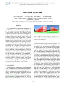
(a)

(b)

(c)

(d)

Figure 1. We propose a novel approach to integrate temporal consistency and local 3D geometry information into CRF image segmentation formulations. ((a) input image; (b) ground truth labels; (c) sematic segmentation results; (d) semantic 3D reconstruction).

acquired at different time steps. It has also been argued that 3D information plays an important role for scene understanding, and several approaches have been developed to estimate 3D information from single 2D images as part of the semantic segmentation process [11, 9, 26, 7]. In parallel, a line of interesting research has emerged on segmentation of 3D point clouds acquired from highly accurate 3D laser range sensors (e.g., Velodyne) [18, 19]. So far, however, there has been no connection between those two research areas. We aim at bridging this gap by incorporating directly estimated 3D information into the 2D image segmentation process. In contrast to [18, 19, 23], we however derive our 3D information from dense stereo depth, which is far noisier than laser data and which therefore requires special provisions. In this paper, we propose a unified framework which incorporates both of those motivations. We introduce a novel CRF framework which forms temporal consistency constraints over consecutive frames through higher-order potentials defined on the points of a local 3D point cloud reconstruction (see Fig. 1(d)). Our framework offers a principled way to incorporate local 3D geometry information

into 2D semantic labeling algorithms. At the same time, the enforced temporal consistency plays an important role in order to smooth the 3D depth measurements over time and thus reduce the noise in 3D estimation. By formulating our model in compliance with the P N based hierarchical CRF framework proposed in [14], we make inference tractable, allowing for efficient Graph-Cuts optimization. As our experiments will show, the resulting model achieves superior segmentation performance on several challenging data sets. The paper is structured as follows. The following section discusses related work. Section 3 gives an overview of CRF-based semantic segmentation methods. Section 4 then presents a detailed description of our novel energy formulation, including two new types of potentials. Finally, Section 5 presents experimental results.

2. Related Work Graphical models, and CRFs in particular, have developed into a remarkable tool for the multi-class image labeling problem. Starting from the influential TextonBoost framework [24], a long line of research has made consistent improvements to the CRF formulation, resulting in considerable advances in the achievable segmentation quality. Especially the recently introduced robust P N potentials [12] and their hierarchical forms [14] are particularly appealing, since they make it possible to capture finer details by enforcing consistency between pixels belonging to the same image segment. Although enforcing higher-order constraints, inference using those potentials is kept tractable within the powerful Graph-Cuts optimization framework. A number of approaches have combined image segmentation with object detection and tracking components to target the scene analysis and scene understanding problems. Geiger et al. [5] proposes a Markov Chain Monte Carlo framework to infer the geometrical and topological properties of the scene together with the semantic activities taking place in the scene. 3D scene geometry is also used in the work of Gupta et al. [9] in the form of physical constraints in an attempt to improve the scene labeling quality by discarding physically implausible environments to be modeled. While there have also been a number of contributions combining segmentation with 3D information, either by integrating monocular structure-from motion (SfM) [25] or stereo disparity [15], none of them explicitly enforces temporal consistency between the subsequent video frames. On the other hand, there has been a lot of work done exclusively in 3D, where the target is to semantically segment 3D point clouds into different classes. Munoz et al. [18] use an Associative Markov Network (AMN) for performing inference in a graph defined over the 3D points using mainly spectral and directional features. Xiong et al. [28] extend the 3D feature set of [18] by computing contextual features over regions of points resulting in improved segmentation

ψc (yc )

ψij (yi , yj )

ψc (yc )

ψi (yi )

Figure 2. Visualization of the CRF framework, with unary potentials ψi , pairwise potentials ψij , and higher-order potentials ψc .

performance. Finally, Shapovalov et al. [23] use structured prediction algorithms to learn class-specific parameters for the pairwise potentials of their Markov network which was defined on the 3D points. In this work we propose a novel framework that combines the advantages of CRF-based approaches in 2D with local 3D information coming from a point-cloud reconstruction. We incorporate temporal consistency constraints within a temporal window by linking corresponding image pixels to the inferred 3D scene point. This formulation allows us to incorporate additional information about the scene content inferred from the point’s 3D neighborhood. Both types of constraints are realized through novel potentials in a CRF formulation.

3. CRFs for Scene Understanding In this section we provide a brief description of the standard CRF model used in multi-class image labeling and of the relevant notation. We closely follow the notation convention used in [13]. Consider a set of target variables Y = {Y1 , ..., Yk }. The CRF is defined on a graph G = (V, E) consisting of N nodes (i.e. |V | = N ), where each node of the graph is represented with a random variable Yk . Each variable Yk ∈ Y is allowed to take values from the discrete domain L = {l1 , l2 , ..., lk }. Therefore, a labeling y = {Yi |i ∈ V } with values lying in L represents a sample from the configuration space YN . The variables Y form a CRF if the probability of a labeling p(y) is strictly positive for all y and p(yi , yE ) = p(yi |yV i ), where E represents the neighboring nodes of i. A CRF is globally conditioned on the set X of observed variables and the distribution p(y|X) is a Gibbs P distribution of the following form: p(y|X) = Z1 exp(− c∈C VC (y)), where Z is a normalization constant, C is the set of maximal cliques in the graph G and VC (y) represents the clique potentials. According to the Maximum A Posteriori (MAP) estimation, the most probable label assignment y ˆ of the CRF is given as the minimum Gibbs energy over the possible labelings y ˆ = arg maxy∈YN p(y|X) = arg miny∈YN E(y). In this paper, we consider P N -based hierarchical CRF

Segment unary Potentials Consistency Potentials 3D unary Potentials

Segment consistency Potentials

Pixel unary Potentials

`

Pairwise potentials

1

k

Figure 3. CRF model. A set of images are optimized together and label consistency is enforced through the temporal consistency potentials which connect the different images through the underlying 3D reconstructions. 3D unary potentials are also added to capture discriminative features of the local geometry around the 3D points.

models as proposed in [12, 14] for the multi-class image labeling problem, whose energy functions E(y) take the following form X X X E(y) = ψi (yi ) + ψij (yi , yj ) + ψc (yc ). (1) i∈V

(i,j)∈E

c∈S

The unary potentials ψi and the pairwise potentials ψij are defined on the pixel level, whereas the higher-order potentials ψc are defined on a set of segments (see Fig. 2). For the unary potentials the TextonBoost framework [24] has been extended similarly to [14] to use multiple features such as SIFT [17], LBP [21], and textons densely extracted from the images. The same framework is used also for the computation of the segment potentials, using the normalized histograms of the dense features [14] as a new feature on the segment level. Finally, for the pairwise potentials a contrast sensitive Potts model [24] is used. This energy formulation in the form of a P N -based hierarchical CRF has shown very good performance in practice. The particular appeal of this model lies in the integration of information from different quantizations of the image space into a unique framework, enabling joint optimization. However, this approach is still working on a single-frame basis, despite the fact that the input is often a video sequence. Furthermore, the above framework is solely based on 2D information coming from image features, ignoring the geometric information of the 3D scene which is in many cases critical in order to achieve a better scene understanding. We believe that temporal consistency should be enforced between consecutive frames and that this could be done in a principled way by estimating the underlying 3D geometry of the scene. Moreover, we argue that the 3D geometry can contribute to the improvement of the segmentation quality as some scene properties have a clear meaning only when a 3D reconstruction is available. In the next section we present our proposed framework, which integrates temporal consistency and scene geometry information in a principled manner in a single CRF.

4. Approach As discussed in the previous section, we propose a novel CRF model which incorporates temporal consistency between consecutive frames and which integrates 3D information from scene geometry. For this, we extend the energy formulation described in Eq. 1 by adding two more types of potentials, temporal consistency potentials and 3D unary potentials (see Fig. 3). In particular, we propose to solve the multi-class image labeling problem for an image by optimizing the semantic labels in a temporal window around the image we are interested in. We then augment the higher-order cliques of the CRF with the sets of pixels that are projections of the same 3D point in different images. Since these new higher-order cliques contain different projections of the same 3D point, the labels of the pixels inside the clique should be consistent. Therefore, it is natural to form a grouping constraint on these pixels which takes the form of a robust P N potential. In addition, we assign a 3D unary potential for each of these higher-order nodes that correspond to different 3D points. This 3D potential allows us to incorporate class-specific information about the possible label of the corresponding 3D point based on the surrounding 3D geometry. Thus, the new energy formulation takes the following form: X X E(y) = ψi (yi ) + ψij (yi , yj ) (2) i∈V

(i,j)∈E

 +miny 

 X

s∈S

ψs (ys ) +

X

ψp (yp ),

p∈P

where ψs denotes the segment potential and ψp is a potential defined over the points of the 3D reconstruction and can incorporate the temporal consistency between frames, as well as local 3D geometry information. Finally, the inference is performed in the CRF using the standard α-expansion algorithm [2, 1, 12]. In order to be able to temporally integrate the semantic information over different frames but to also exploit the in-

formation coming from 3D scene geometry, we compute a point cloud reconstruction of the environment. Our reconstruction pipeline consists of 3 major components: visual odometry, stereo depth estimation and 3D reconstruction. Visual odometry. In order to fuse the individual disparity maps to a consistent 3D point cloud reconstruction, we estimate the camera position and rotation P = (R, t) for each frame using visual odometry (VO). For this, we use a stereo VO pipeline, as proposed by Nister [20]. We maintain the uncertainty about the camera pose with a Kalman filter, which also helps us smooth the VO calculations. Stereo depth estimation. In this component we compute the stereo disparity maps individually for each of the frames of the sequence using the ELAS algorithm, as described in [6]. ELAS provides high quality depth maps at a low computational cost and it is thus suitable for our application. 3D reconstruction. In the last component of our pipeline, we fuse the 3D points from the individual depth maps into a common 3D reconstruction using the visual odometry information. In the first frame of the sequence, we create an initial point cloud by generating a 3D point for each of the image pixels for which we are given a valid disparity from the stereo depth estimation. Each of the 3D points is associated with a zero-velocity Kalman filter that keeps track of its localization uncertainty. The uncertainty covariance of a reconstructed 3D point can be computed using forward error propagation [10] as    T   σu 0 0 ∂fb  0 σv 0  ∂fb , (3) C= ∂u ∂u 0 0 σd where σu , σv and σd are the standard deviations in the two image dimensions and in the disparity, respectively, and fb represents the backprojection function   u B fb (u, v, d) =  vsvu  . (4) d fu u and v are the pixel coordinates, fu is the focal length of the camera in pixels, B is the baseline, d is the disparity, and svu is the skew parameter of the camera. Once an initial point cloud has been created, we project its points into each of the following frames after incorporating the estimated camera motion. In this way, we create a virtual disparity dv for each point, which is then compared with the disparity computed from the stereo depth estimation module d on this specific pixel. If |dvd−d| is below a certain threshold td , the 3D point is associated with this pixel and its Kalman filter is updated according to the new measurement. For all image pixels that we cannot associate with existing 3D points, we generate new 3D points that are added to the point cloud. This results in a robust 3D integration for static scene structures. For all further processing steps, we

Figure 4. Visualization of the 3D Features (a) Height (h) above the estimated ground plane; (b) Point-ness (λ0 ); (c) Linear-ness (λ0 − λ1 ); (d) Surface-ness (λ1 − λ2 ); (e) Cosines of the angles between the normal and the tangent vectors to the horizontal plane; (f) Dimensions of the oriented bounding box along the principal components axes.

keep only those 3D points whose localization uncertainty surpasses a threshold. Temporal Consistency Potentials. The consistency potentials take the form of robust P N potentials [12] and their role is to force the labels of the pixels that correspond to the same 3D point to have the same label. The new node that is constructed is allowed to take a label from the same label set as the segment potentials. The idea behind this is to collect the opinions of the pixels of different frames for the same 3D point. Therefore, the consistency potential ψp (yp ) is defined as follows ψp (yp ) = min (γpmax , γpl + kpl Npl ) , l∈L X l γp = λs |p| min( wci ψi (yi ) + K, α)

(5) (6)

i∈p

γpmax = |p|(λp + λs α),

(7)

where α is a truncation threshold, K is a normalizing conP stant, and Npl = i∈p δ(yi 6= l) is the number of pixels disagreeing with the majority vote. Finally, the parameter wci weights the different frames’ contributions to the clique. 3D Potentials. The 3D potentials are an extension of the consistency potentials. They enable us to integrate classspecific information from the local geometry around each of the 3D points. They take the following form: ψp (yp ) = min (γpmax , γpl + kpl Npl ), l∈L  X γpl = λs |p| min  wci ψi (yi ) i∈p

+wp3D (−log(Hl (p))) + K, α

(8) (9) ! ,

where Hl (p) is the response of a classifier which indicates the probability for a 3D point clique to take a certain label. We use the output of a Randomized Decision Forests classifier [8] to define the 3D potentials. Since we collect

the output of multiple trees, we assign the value of the potential function for a specific class to be proportional to the number of trees that have voted for this class. Often, the amount of training data that we have is significantly biased towards some of the classes. To alleviate this effect, we randomly subsample the points of the different classes proportionally to the class frequency in order to create a balanced training set with regard to the different classes and thus achieve an unbiased classification result [3]. We have implemented a number of local geometric features that are extracted from the 3D point cloud and are then fed into the classifier. Firstly, we make use of the height of a 3D point above the local ground plane (Fig. 4(a)), which is estimated during visual odometry computation. Secondly, we compute the spectral (Fig. 4(b,c,d)) and directional features (Fig. 4(e)) proposed by Munoz et al. [18], and finally we compute the dimensions of the oriented bounding box that encloses the neighborhood of each point in the three principal components space [19] (Fig. 4(f)). The resulting feature vector consists of 8 dimensions in total and the computation of the 3D features used the PCL library [22].

5. Experimental Results Datasets. We evaluate our method on two datasets: the L EUVEN stereo dataset [15] and the C ITY stereo dataset [4]. The L EUVEN dataset was first used in [16]. It consists of 1175 image pairs captured at 25fps with a resolution of 360x288 pixels over a driving distance of about 500m. Recently, a subset of this dataset has been enriched with object class segmentation annotations [15]. The augmented subset contains 70 images divided into 50 training and 20 test frames with a cropped resolution of 316x256. Each pixel is manually labeled to one of the 8 class labels defined in [15]. The C ITY dataset contains 3000 image pairs of high quality 13 Hz footage at 640x480 pixel resolution. The video was captured by a moving vehicle inside the city center of Zurich. The C ITY dataset is part of the Z URICH corpus [4] of datasets which is divided into several subsequences captured at daylight and dusk. Ground truth labeled frames are provided for sporadic images along the several datasets. In addition, we have augmented the dataset with 30 segmentation annotations for the C ITY sequence. This resulted in a total of 71 ground truth images used for training and 32 for testing. The pixels in the annotated frames take one of the 13 label classes defined in [4]. L EUVEN dataset. In a first quantitative experiment we assess the improvement in performance our proposed potentials bring. We compare a baseline system which implements a basic version of the energy formulation of Eq. 1 to two versions of our proposed framework. In the first version, only the temporal consistency potentials are added, whereas in the second both the temporal consistency and the 3D potentials are included. Except where noted otherwise,

we use a temporal window of 5 frames, the different frames contribute equally to the consistency potentials, the weighting factors between the potentials are wci = 0.7, wp3D = 0.3, and a forest of 20 trees of depth up to 10 levels is used for evaluating the 3D unary potentials. As can be seen in Table 1, the introduction of the temporal consistency potentials consistently improves performance across all object classes and all evaluation measures. In particular, the global recall is improved by 1.8% and the average recall by 3.4%, showing the advantage of the proposed approach. The 3D unary potentials bring an additional improvement in the global accuracy and for some of the classes (e.g., building, sidewalk) using the recall measure, but they improve the results for almost all classes for the IvsU measure. Note that the quality of the images in this dataset is rather low and the corresponding 3D reconstruction therefore contains a high level of noise, which limits the improvements the 3D potentials can bring here. All of the above findings are also nicely illustrated in the confusion matrices in Fig. 5 and in the perceived quality of the segmentation images in Fig. 6. In a second round of more in-depth experiments on this dataset we evaluated how the size of the temporal window around the image of interest affects segmentation performance. We found that the performance is practically not affected: a temporal window of 3 frames achieves a global recall of 95.1%, in comparison to 95.2% for the 5- and 7-frames windows. We also assessed the achievable segmentation performance when keeping the system causal (i.e., when choosing the reference frame to be at the end of the temporal window, such that no look-ahead into future frames is used). Such a change results in a slight drop of 0.3% in global recall compared to the centered setting, but it still constitutes a 1.5% improvement over the baseline. Finally, we show a comparison to the recent approach of [15] using their evaluation procedure, which discards the person category (Tab. 1). The results are comparable, even though [15] use a more complicated model (3 levels of hierarchy and pairwise connections in all hierarchies). C ITY dataset. Since the Leuven dataset consists of lowresolution images, the resulting depth maps and 3D reconstructions are of poor quality, including a substantial amount of noise. Therefore, we also evaluate our approach on the C ITY dataset, which has higher resolution images leading to better 3D reconstructions. Again, we begin with a comparison to the baseline system to assess the performance improvement of the temporal consistency and the 3D potentials. Except where noted otherwise, we use a temporal window of 3 frames, the different frames contribute equally to the consistency potentials, the weighting factors between the potentials are wci = 0.8, wp3D = 0.2, and a forest of 50 trees of depth up to 10 levels is used for evaluating the 3D unary potentials.

(a)

(b)

(c)

Figure 5. L EUVEN : Confusion matrices for different energy formulations. (a) Baseline. (b) Consistency potentials (c) Consistency potentials and 3D unary potentials. As it can be seen the introduced potentials improve the performance consistently over the baseline system. The low performance across all the systems on the person class can be explained by the fact that there are very few instances in the test set and they are often heavily occluded. Furthermore, no object detections are used in this CRF formulation.

(a)

(b)

(c)

(d)

(e)

Figure 6. L EUVEN : Qualitative results (a) Test images; (b) ground truth labeled images; (c) segmentations obtained using the baseline approach; (d) segmentations obtained using consistency potentials; (e) segmentations obtained using consistency potentials and 3D unary potentials. The introduced potentials improve the image labeling quality significantly. (Best viewed in color)

As shown in Table 2, the consistency potentials improve the global recall by 1.6% and the average recall by 2.4%. The improvement is again consistent over all the classes (except for the sign class), with significant improvements for some classes. In particular for the mark class, there is an increase of 13.2% in recall, which also becomes visible in the qualitative results of Fig. 8. The 3D potentials improve the summary scores of global and average for both evaluation measures. It should be noted here that some of the classes have a distinctive geometry and can therefore be classified more easily (e.g., curb), whereas others have very similar geometrical properties (e.g., mark and road). In addition, some of the object classes represent mobile objects (e.g., car). For these classes the reconstruction becomes difficult and often fails to recover the original object shape. This can explain the slightly worse performance of the 3D potentials for some of the classes. A more detailed overview is available from the confusion matrices in Fig. 7. It should also be noted that the wall and grass classes occur only very rarely in the test images. We decided to keep them in our

result tables to be consistent with [4] and since they were used for the training, but we think that they should be either omitted (grass) or be merged with other classes (wall with building) since those classes are almost indistinguishable. Finally, we tried to compare our approach’s performance to the one reported in [4]. Although a direct comparison to [4] is impossible due to the diverging training and test sets, it is interesting to observe that our approach improves both on their reported summary performances (with 57.6% vs. 45.2% average recall) and on every single class except for street markings and poles, where their results are 3% and 5% higher, respectively. As can also be observed in Fig 9, our segmentation is far more detailed and accurate.

6. Conclusions and Future Work We have presented a novel framework for enforcing temporal consistency between consecutive videos frames in a semantic segmentation application. Our proposed method makes it possible to also incorporate semantic information coming from local 3D geometric features in a single energy

Building

Sky

Car

Person

Road

Sidewalk

Bike

Global

Average

Recall Baseline Temp. Cons. Temp. Cons. + 3D Joint segmentation and depth [15] Temp. Cons. + 3D Intersections vs Union Baseline Temp. Cons. Temp. Cons. + 3D

95.4 96.6 97.8 96.7 97.9

96.9 98.7 97.1 99.8 97.1

84.7 86.7 85.4 94.0 85.4

0.0 0.0 0.0 -

96.3 98.5 98.4 98.9 98.4

47.3 55.8 56.1 60.6 56.1

50.8 59.6 59.3 59.5 59.3

93.0 94.8 95.2 95.8 95.4

67.4 70.8 70.6 84.9 82.4

93.1 94.8 95.2

87.0 90.6 92.9

65.6 75.0 75.5

0.0 0.0 0.0

90.5 92.5 93.0

43.7 51.4 52.2

47.5 55.9 55.7

-

61.1 65.7 66.4

Table 1. L EUVEN : Quantitative results. The evaluation measures are defined in [14]. The two proposed formulations improve the performance consistently for the individual classes and the overall scores. Note that there are very few person instances in the test set.

(b)

(a)

(c)

Figure 7. C ITY: Confusion matrices for different energy formulations. (a) Baseline. (b) Consistency potentials (c) Consistency potentials and 3D unary potentials. As can be seen, the introduced potentials improve the performance consistently over the baseline system. The low performance on the wall and grass classes can be explained by the very few instances of those classes in the test set.

(a)

(b)

(c)

Figure 9. Comparison with [4]: (a) Test image. (b) Result from [4]. (c) Our result. Our system achieves a much more detailed and accurate labeling. (Best viewed in color)

minimization formulation. We have evaluated our approach on two stereo sequences taken from mobile platforms. Our results show that our method achieves improved segmentation performance compared to an image-only baseline and that it generalizes well to varying image conditions. In future work, we plan to investigate better 3D features that are better adapted to the noisy stereo depth data. In addition, we will explore how class-specific information obtained from the segmentations can be used to improve 3D integration for the movable object categories. Acknowledgements. This project has been funded, in parts, by the EU project EUROPA (ICT-2008-231888) and the cluster of excellence UMIC (DFG EXC 89).

References [1] Y. Boykov and V. Kolmogorov. An experimental comparison of min-cut/max-flow algorithms for energy minimization in vision. PAMI, 26(9):1124–1137, 2004. [2] Y. Boykov, O. Veksler, and R. Zabih. Fast approximate energy minimization via graph cuts. PAMI, 23(11):1222–1239,

2002. [3] C. Elkan. The foundations of cost-sensitive learning. In IJCAI, 2001. [4] A. Ess, T. Mueller, H. Grabner, and L. van Gool. Segmentation-Based Urban Traffic Scene Understanding. In BMVC, 2009. [5] A. Geiger, M. Lauer, and R. Urtasun. A Generative Model for 3D Urban Scene Understanding from Movable Platforms. In CVPR, 2011. [6] A. Geiger, M. Roser, and R. Urtasun. Efficient Large-Scale Stereo Matching. In ACCV, 2010. [7] A. Geiger, C. Wojek, and R. Urtasun. Joint 3D Estimation of Objects and Scene Layout. In NIPS, 2011. [8] P. Geurts, D. Ernst, and L. Wehenkel. Extremely randomized trees. Machine Learning, 63(1):3–42, 2006. [9] A. Gupta, A. Efros, and M. Hebert. Blocks world revisited: Image understanding using qualitative geometry and mechanics. In ECCV, 2010. [10] R. I. Hartley and A. Zisserman. Multiple View Geometry in Computer Vision. Cambridge University Press, 2004. [11] D. Hoiem, A. Efros, and M. Hebert. Geometric Context from a Single Image. In ICCV, 2005. [12] P. Kohli, L. Ladick`y, and P. Torr. Robust higher order potentials for enforcing label consistency. IJCV, 82(3):302–324, 2009. [13] D. Koller and N. Friedman. Probabilistic graphical models. MIT Press, 2009. [14] L. Ladick`y, C. Russell, P. Kohli, and P. Torr. Associative hierarchical crfs for object class image segmentation. In ICCV, 2009.

(a)

(b)

(c)

(d)

(e)

Road

Mark

Building

Sidewalk

Tree/Bush

Pole

Sign

Person

Wall

Sky

Curb

Grass

Global

Average

Recall Baseline Temp. Cons. 3D + Temp. Cons. Intersections vs Union Baseline Temp. Cons. 3D + Temp. Cons.

Car

Figure 8. C ITY: Qualitative results (a) Test images. (b) Ground truth labeled images. (c) Segmentations obtained using the baseline approach. (d) Segmentations obtained using consistency potentials. (e) Segmentations obtained using consistency potentials and 3D unary potentials. The introduced potentials improve the image labeling quality significantly. (Best viewed in color)

74.5 78.2 77.1

97.6 98.2 97.8

54.1 67.3 70.0

91.6 92.6 92.6

59.6 66.1 65.8

82.5 87.1 86.9

4.2 2.8 4.5

54.5 50.2 50.9

60.3 65.4 66.1

0.0 0.0 0.0

98.3 98.6 98.6

35.7 37.5 38.3

0.0 0.0 0.0

89.5 91.1 91.2

54.8 57.2 57.6

58.6 62.1 61.9

90.3 92.4 92.5

52.3 61.7 65.9

85.2 86.8 87.3

42.6 50.0 48.8

71.9 77.5 77.7

3.8 2.7 4.2

47.2 42.4 45.4

41.7 43.1 43.1

0.0 0.0 0.0

92.3 93.8 92.7

32.5 34.0 32.8

0.0 0.0 0.0

-

47.6 49.7 50.2

Table 2. C ITY: Quantitative results. The evaluation measures as defined in [14]. It can be seen that the two proposed formulations improve the performance consistently in the individual and overall scores. The wall and grass classes appear almost nowhere in the test set. [15] L. Ladick`y, P. Sturgess, C. Russell, S. Sengupta, Y. Bastanlar, W. Clocksin, and P. Torr. Joint optimization for object class segmentation and dense stereo reconstruction. IJCV, pages 1–12, 2010. [16] B. Leibe, N. Cornelis, K. Cornelis, and L. Van Gool. Dynamic 3d scene analysis from a moving vehicle. In CVPR, 2007. [17] D. Lowe. Distinctive image features from scale-invariant keypoints. IJCV, 60(2):91–110, 2004. [18] D. Munoz, N. Vandapel, and M. Hebert. Directional Associative Markov Network for 3-D Point Cloud Classification. In 3DPVT, 2008. [19] D. Munoz, N. Vandapel, and M. Hebert. Onboard contextual classification of 3-d point clouds with learned high-order markov random fields. In ICRA, 2009. [20] D. Nist´er, O. Naroditsky, and J. Bergen. Visual odometry for ground vehicle applications. Journal of Field Robotics, 23(1):3–20, 2006. [21] T. Ojala, M. Pietik¨ainen, and D. Harwood. A comparative study of texture measures with classification based on featured distributions. Pattern Recognition, 29(1):51–59, 1996.

[22] R. Rusu and S. Cousins. 3d is here: Point cloud library (pcl). In ICRA, 2011. [23] R. Shapovalov and A. Velizhev. Cutting-Plane Training of Non-associative Markov Network for 3D Point Cloud Segmentation. In 3DPVT, 2011. [24] J. Shotton, J. Winn, C. Rother, and A. Criminisi. Textonboost for image understanding: Multi-class object recognition and segmentation by jointly modeling texture, layout, and context. IJCV, 81(1):2–23, 2009. [25] P. Sturgess, K. Alahari, L. Ladick`y, and P. Torr. Combining appearance and structure from motion features for road scene understanding. In BMVC, 2009. [26] J. Tighe and S. Lazebnik. Understanding Scenes on Many Levels. In ICCV, 2011. [27] C. Wojek and B. Schiele. A Dynamic Conditional Random Field Model for Joint Labeling of Object and Scene Classes. In ECCV, 2008. [28] X. Xiong, D. Munoz, J. Bagnell, and M. Hebert. 3-D Scene Analysis via Sequenced Predictions over Points and Regions. In ICRA, 2011.