In order to optimize revenue, service firms must integrate within their pricing poli- ... flights (direct or through a hub-and-spoke network) must take into account the.
Joint Design and Pricing on a Network Martine Labb´e 2 Patrice Marcotte 3 Gilles Savard 4 1 LAMIH/ ROI, Universit´e de Valenciennes 2 SMG and ISRO, Universit´e libre de Bruxelles 3 CRT and D´epartement d’Informatique et de Recherche Op´erationnelle Universit´e de Montr´eal 4 GERAD and D´epartement de Math´ematiques et de G´enie Industriel Ecole Polytechnique de Montr´eal Luce Brotcorne
1
Abstract In order to optimize revenue, service firms must integrate within their pricing policies the rational reaction of customers to their price schedules. In the airline or telecommunication industry, this process is all the more complex due to interactions resulting from the structure of the supply network. In this paper we consider a streamlined version of this situation where a firm’s decision variables involve both prices and investments. We model this situation as joint design and pricing problem which we formulate as a mixed-integer bilevel program. Next, we develop an algorithmic framework based on the novel application of Lagrangian relaxation to bilevel programs. Numerical results show that our procedure is capable of solving problems of significant sizes.
1
Introduction
This paper is devoted to a model that captures the interaction between system design, price setting and consumer choice over a transportation network. The problem involves two decision makers acting non cooperatively and in a sequential way. The upper level (leader) strives to maximize its revenue raised from tariffs imposed on a set of goods or services in its control, while the lower level (follower) optimizes its own objective, taking into account the tariff schedule set by the leader. The leader explicitly incorporates the reaction of the follower in his optimization process. In the field of economics, this fits the principal/agent paradigm (Van Ackere [11]) where the principal, fully aware of the agent’s rational behaviour, induces cooperation from the agent through an incentive scheme. In the field of mathematical programming this problem belongs to the class of bilevel optimization problems with bilinear objectives at both levels of decision. In the current context of deregulation, pricing decisions have become crucial for airline, trucking, telecommunication and service industries where intense price competition and 1
network modifications have occurred. Clearly a profit maximizing firm must consider the trade off between the cost of service and the revenue generated when designing its system and prices. In the passenger or freight airline industry, a carrier (the leader) selects routing patterns, flight schedules and fares. For instance, Budenbender et al. [5] describe a system where freight providers such as express shipment companies operate or rent an aircraft fleet that must provide a high level of service. For consolidation purposes, the freight is first shipped to an airport, next it is flown non-stop to another airport, finally to be loaded on trucks and shipped to its final destination. The problem then consists in determining the terminal to operate, the take-off time, the transportation of the freight to an airport and the rate that will be charged. In passenger transportation, the introduction of new flights (direct or through a hub-and-spoke network) must take into account the supply over the entire network of flights, both from the leader airline and its competitors. The decisions are then taken with respect to the incurred costs, the quality of service, the possible influence on demand to other destinations and, most important, the revenues generated by the new services (Lederer [9], [10]). In the surface freight transportation industry, important structural changes occur as shippers optimize the end-to-end supply through the implementation of web-based portals. In that context, the costs incurred by a carrier is made up of two components: a fixed cost (including trade compliance, trade settlement with country-specific international trading portals, multimodal aspects, operating resources costs, global handling costs, etc.) and a unit transportation cost (Kerr [6]). Upon reception, a service carrier (the leader) has to decide whether or not to accept a request and, if accepted, to set a price. In reaction to those prices, the shippers (the follower) want their goods be transshipped at minimal cost, hence the bilevel structure of the problem. In the telecommunication area, a service provider (the leader) has to make network deployment decisions and to set prices for bandwidth usage. The response of users (the follower) to prices induces traffic on the network. In the current deregulated markets, pricing is a fundamental issue for communications carriers. Indeed, as new systems of ever larger capacities are introduced, the marginal cost of data transmission is rapidly decreasing. Exploiting those cost savings and handling increased demand involves the optimization of technology acquisition and pricing processes (Lanning et al. [8] and Ba¸sar and Srikant [1]). Design and pricing are also challenging issues for business information service providers [2]. Information agencies such as Reuters and Bloomberg (foreign currency markets) and Aspect Development (component information services) are essentially intermediates between firms that generate and firms that use content. As information service providers (the leader) incur large fixed costs (data entry and updates, software development, database management systems, connections to commercial networks), their problem consists in specifying the size of the database they provide to subscribers (followers) as well as the price they will charge for subscriptions. At the lower level, the subscribers adapt their usage volume according to the level of service and tariffs of the service providers, or yet may select the self-service option whereby they collect and collate information directly from the sources.
2
Until now, design and pricing issues have mostly been treated separately. However, they are intrinsically linked and have to be addressed jointly. To our knowledge the only papers addressing the joint design and pricing problem are those of Lederer [9], Ba¸sar and Srikant [1] and Bashyam [2]. Lederer [9] proposes a Nash equilibrium model of air transport competition where firms select routes and prices. Competition is studied under two different assumptions about consumers’ choice: either they can bundle individually purchased services, or they cannot. The paper, which focuses on the existence issue, does not provide solution algorithms. Consumer demand is provided by demand functions that are exogenous to the model. Ba¸sar and Srikant [1] study the economics of providing large capacity from a telecommunication provider’s point of view. Design choices are not modelled using binary decisions but through continuous capacity variables. Each user is charged a fixed price per unit of bandwidth used, and this price is independent from congestion. The transmission rate of each user is assumed to be a function of network congestion and price per unit of bandwidth. The aim of the service provider is to maximize its revenue. The authors show that, as the number of users increases, the optimal price per unit of bandwidth charged by the service provider may increase or decrease depending upon the bandwidth of the link. However, for all values of the link capacity, the overall performance of each user improves and the service provider’s revenue per unit of bandwidth increases, thus providing an incentive for the service provider to increase the available bandwidth in proportion to traffic. Although this work provides some theoretically insight into the problem, no computational procedure is described for its solution. Bashyam [2] analyzes service design and pricing of business information services in a competitive environment, using game-theoretic concepts. The problem consists in determining the optimal size of the database, as well as the subscription price they will fix for subscriptions, taking into account the reaction of subscribers who want to minimize their cost. They consider two types of interactions: monopoly or duopoly, and two types of information delivery technologies: online service that allows subscribers to access information over online networks, and package service that delivers information using physical media such as CD-ROM’s. Their analytical approach investigates the differences in price structure associated with the type of provided services. In the case of duopoly, they also analyze the class of consumers (high or low volume consumers) served depending on the size of the database and on prices. In this paper we focus on a joint design and pricing problem on networks involving multicommodity flows. The upper level is concerned with maximizing profit raised from tariffs set on a subset of arcs which is determined by the leader. This problem can be adequately represented as a bilevel program and constitutes an extension of the model proposed by Brotcorne et al [3] and [4] for the determination of optimal tariffs on a singlecommodity, respectively multicommodity, transportation network. The specificity of the problem considered here consists in simultaneously determining which connections are opened and which tariff policy is applied. This differs from our previous work where only tariff schedule was subject to optimization. The outline of this paper is as follows. In Section 2, we introduce a mixed-integer bilinear formulation for the joint design and pricing problem and discuss its properties.
3
In Section 3, we prove that some lower level constraints can be moved to the first level, thus reducing the size of the problem. In Section 4, we describe a solution algorithm. Finally numerical results are presented and analyzed in Section 5.
2
A joint design and pricing model
Let us consider a network based on the underlying graph G = (N, A), with node set N and arc set A. A node represents either a supply site, a demand site, or the endpoints of an arc on which goods are carried. The set of arcs is partitioned into two subsets A1 and A2 where A1 denotes the set of links operated by the leader and A2 the set of links operated by its competitors. With each arc a ∈ A1 , we associate a tariff Ta , to be determined by the leader, a fixed opening cost fa and an operating cost ca charged to the leader. Arcs in A2 are tariff-free and only bear a unit cost da which is outside the control of the leader. Demand is modelled by a set K of commodities. These may represent distinct physical goods or identical physical goods associated with different points of origin and destination. Each commodity is associated with an origin-destination pair (o(k),d(k)). The demand vector bk corresponding to commodity k is specified by: bki =
k n
if i = o(k), −nk if i = d(k), 0 otherwise,
where nk represents the amount of flow of commodity k to be shipped from o(k) to d(k). The variable xka (respectively yak ) denotes the flow of commodity k on arc a ∈ A1 (respectively a ∈ A2 ). The binary variable va , associated with each arc a ∈ A1 , indicates whether (va = 1) or not (va = 0) arc a belongs to the network design. The leader’s variables are either discrete (design variables) or real-valued (tariffs). Lower level variables, i.e., flows, are real-valued. Based on the above notation, the joint design and pricing problem can be formulated as a mixed bilevel program with bilinear objectives and linear constraints. The commodity flows xka and yak correspond to an optimal solution of the lower level linear program parameterized by the upper level tariffs Ta , which is solved on the sub-network resulting from the binary variables va : (JDP) max T,v
X X k∈K a∈A1
Ta xka −
X a∈A1
fa va −
X X k∈K a∈A1
ca xka
s.t. va ∈ {0, 1}
(1) ∀a ∈ A1 ,
(2)
where (x, y) is an optimal solution of min x,y
X X
(
Ta xka +
k∈K a∈A1 k k
X a∈A2
da yak )
s.t. Ax + By = bk xka ≤ nk va xk , y k ≥ 0
(3) ∀k ∈ K, ∀k ∈ K ∀a ∈ A1 , ∀k ∈ K.
4
(4) (5)
The upper level objective (1) is to maximize total net revenue and is expressed as the difference between the sum of revenues arising from tariffs Ta and the sum of fixed opening costs and operating costs. The objective of the lower level problem (3) is to minimize the total cost of the paths selected by network users. Constraints (5) state that arcs can only be used if they are open. Constraints (4) represent the flow balance equations. For specific tariff levels and design variables, the flow repartition for the lower level problem is given by shortest origin-destination paths on the sub-network composed of tariff-free and tariff arcs that are open. We assume that, given the choice between paths of equal cost, the path selected is the one yielding the highest profit for the leader. As in Labb´e et al. [7], we also assume that: • there cannot exist a tariff schedule that generates profits and simultaneously creates a negative cost cycle in the network, • there exists at least one path composed of tariff-free arcs for each origin-destination pair. These assumptions imply that the lower level optimal solution corresponds to a set of shortest paths, and that the upper level profit is bounded from above. A feasible upper bound on the profit is provided by the following proposition. Proposition 1. An upper bound on the leader’s profit is the difference between the follower’s optimal objective corresponding to infinite tariffs, and the optimum value of the classical network design problem obtained by setting tariffs at zero. Proof Let us perform the change of variable T 0 = T − c, which is tantamount to setting the usage cost of every tariff link a ∈ A1 to ca at the lower level. For fixed design vector v, the resulting problem is of the form considered by Labb´e et al. [7], who derived the valid upper bound U − L(v), where U denotes the cost of a lower level solution when access to tariff arcs is denied (infinite tariffs), and L(v) is the cost of a shortest path solution with Ta0 = 0 and cost set to ca on each link a ∈ A1 . It follows that a valid bound for the value of an optimal solution to JDP is given by {U − L(v)} = U − min {L(v)}, max v v
(6) 2
as claimed. Example
The example of Figure 1 shows that the upper bound need not be reached. In this example, demand is set to 2 on origin-destination pair 1-2 and to 4 on pair 3-4, while (5,6) is the sole tariff link. Fixed opening and operating costs for the leader are set, respectively, to 1 and 0. The optimal solution, corresponding to a profit of 11 units is reached for T5,6 = 2. However the upper bound on the profit is equal to 40 − 21 = 19. 2
5
8
1
2
1
2
T 56
5
6
3
1
3
4
6
Figure 1: Upper bound on profit not reached at the optimal solution. Now, taken into account that the entire demand associated with a given OD pair can be assigned to a single shortest path, one can, without loss of generality, reformulate JDP as: max T,v
X X a∈A1 k∈K
nk Ta xka −
X a∈A1
fa va −
X X a∈A1 k∈K
nk ca xka
s.t. va ∈ {0, 1} min x,y
X k∈K k
nk (
X
a∈A1 k
∀a ∈ A1 , Ta xka +
X a∈A2
da yak )
k
∀k ∈ K, ∀a ∈ A1 ∀k ∈ K, ∀k ∈ K,
s.t Ax + By = e xka ≤ va xk , y k ≥ 0 where
eki
1
(7)
if i = o(k),
= −1 if i = d(k), 0
otherwise.
For fixed design vector v, the resulting problem reduces to a multicommodity toll optimization problem that can be reformulated as a mixed integer program (see Brotcorne et al. [4]). This formulation readily extends to a MIP formulation for JDP through incorporation of the design variables va . In Section 5 (Numerical Results), this formulation is solved using the commercial software CPLEX and serves as a testbed for our method, on small problem instances. 6
In the case where there is only one OD pair, JDP reduces to the toll optimization problem analyzed by Brotcorne et al. ([3], [4]). Indeed, the binary flow variables xa can then replace the design variables va , and the problem formulation becomes: max T,x
s.t. min x,y
X a∈A1
nTa xa −
X a∈A1
fa xa −
X a∈A1
nca xa
xa ∈ {0, 1} n(
X
a∈A1
Ta xa +
∀a ∈ A1 , X a∈A2
da ya )
Ax + By = e, x, y ≥ 0. Next one defines modified tariffs Tea = Ta − n1 fa − ca and obtains the toll optimization problem: max T˜
min x,y
s.t.
X a∈A1
X a∈A1
nT˜a xa (T˜a + ca + fa /n)xa +
X a∈A2
da ya
Ax + By = e, x, y ≥ 0.
Note that dropping the flow integrality constraints at the upper level is justified by the fact that the lower level constraints are totally unimodular and that it is not in the interest of the leader to induce noninteger (split) flows.
3
Moving constraints from the lower to the upper level
For general bilevel programs, constraints involving both upper and lower level variables cannot be moved freely from one level to the other, without altering both the feasible set and the optimal solution of the bilevel program. Upper level constraints are transparent to the follower, and can only be induced through a proper choice of the leader’s tariffs. By transferring them to the lower level, we obtain a relaxation of the original program.1 It is a remarkable feature of JDP, and the wider class of bilinear bilevel programs to which it belongs, that one can perform this operation, which will be exploited in the design of a solution algorithm. Proposition 2. Let x, T , c ∈ IRm1 , y, d ∈ IRm2 , b1 ∈ IRn , b2 a vector of positive components in IRr , A, B ∈ IRm2×n and A2 a nonnegative matrix in IRr×m1 . Then the following bilinear bilevel programs are equivalent, in the sense that an optimal solution 1
Even in the simpler case of linear bilevel programming, the feasible set corresponding to joint upper level constraints may be disconnected.
7
to P1 can be matched to a feasible solution of P2 with the same objective value, and vice versa. (P1) max T x
(P2) max T x
T
min x,y s.t.
T
A2 x ≤ b 2 ,
(T + c)x + dy min x,y
A1 x + By = b1 , A2 x ≤ b2 , x, y ≥ 0,
s.t.
(T + c)x + dy A1 x + By = b1 , x, y ≥ 0.
Proof Let us replace the lower level problems of P1 and P2 by their respective primal-dual optimality conditions, where λ and δ are the dual variables associated with constraints of P1 and their equivalent in P2. This yields (P10 )
max
T,x,y,λ,δ
s.t.
(P20 )
Tx 1
1
A x + By = b , A2 x ≤ b2 , λA1 + δA2 ≤ c + T, λB ≤ d, (d − λB)y = 0, (c + T − λA1 − δA2 )x = 0, δ(b2 − A2 x) = 0, x, y ≥ 0, δ ≤ 0.
max
Tx
s.t.
A1 x + By = b, A2 x ≤ b 2 , λA1 ≤ c + T, λB ≤ d, (d − λB)y = 0, (c + T − λA1 )x = 0, x, y ≥ 0.
T,x,y,λ
Let (T ? , x? , y ? , λ? ) be an optimal solution of P20 . By setting δ ? = 0, one obtains a solution (T ? , x? , y ? , λ? , 0) of P10 with the same objective value. Conversely, let (T ? , x? , y ? , λ? , δ ? ) be an optimal solution of P10 . We want to show that δ = 0 and thus (T ? , x? , y ? , λ? , δ ? ) is an optimal solution of P20 as well. Let us assume, by P contradiction, that there exists an index i ≤ r such that δi? < 0, then 0 < b2i = j a2ij x?j . As x?j ≥ 0 for all j it follows that there exists an index j such that both x?j and a2ij are positive. P Then, from complementarity slackness, we have that cj + Tj? − [λ? A1 ]j − l δl? a2lj = 0. ?
P
Let us set Tj0 = Tj? − l δl? a2lj and δj0 = 0. Since A2 is nonnegative, δ ? ≤ 0 and δi? a2ij < 0, we obtain that Tj0 > Tj? . Finally, by setting Tl0 = Tl? and δl0 = δl? for all l 6= j, we conclude that (T 0 , x? , y ? , λ? , δ 0 ) is still a feasible solution for P1 with higher objective value T 0 x? . 2 This contradicts the optimality of (T ? , x? , y ? , λ? , δ ? ) and concludes the proof.
8
Corollary 1. The capacity constraints (5) of JDP can be moved to the upper level. Proof It is sufficient to show that, for fixed design vector v, the resulting pricing problem can be written in the format P1. This is achieved, very simply, by introducing total arc flow variables X xa = xka . k∈K
The resulting bilevel program is: max T
min x,y
X a∈A1
X
a∈A1
Ta xa − Ta xa +
X a∈A1
c a xa
X
da ya a∈A2 k k
Axk + By = b xka ≤ nk va X xa = xka
∀k ∈ K, ∀k ∈ K ∀a ∈ A1 , ∀a ∈ A1 ,
k∈K
X
yak
∀a ∈ A2 ,
xk , y ≥ 0
∀k ∈ K,
ya =
k∈K k
which is in the required format, with the obvious correspondences between vectors and matrices. 2
4
A solution procedure for JDP
The difficulty in solving JDP is twofold: the presence of binary variables and the complementarity constraints arising in the optimality conditions of the lower level linear program. In this section, we propose an iterative algorithm that adapts Lagrangian relaxation to the bilevel framework. We treat constraints (7) as the ‘complicating’ ones; these are appended to the objective to form the usual Lagrangian function. To evaluate the dual function, one has to solve the Lagrangian subproblem, itself an NP-hard toll optimization problem. This latter problem is solved using a variant of the primal-dual algorithm proposed in Brotcorne et al [3]. More precisely, the subproblem is reformulated as a single level bilinear problem through the use of an exact penalty function applied to the lower level complementarity term. Next, we update sequentially the upper and lower level variables, increasing the penalty parameter when no progress is achieved. Whenever a basis change occurs at the lower level, tariffs that are optimal with respect to the new bases are computed. This ‘inverse optimization’ procedure actually solves a modified multicommodity flow problem. Let us now detail the procedure. The dual function, for a given nonnegative vector u, is obtained by solving the bilevel program: (LSP(u))
L(u) =
max
T,v,x,y,λ
X X
a∈A1 k∈K
nk Ta xka − 9
X
a∈A1
fa va −
X X
a∈A1 k∈K
nk ca xka
+
X X a∈A1 k∈K
uka (va − xka )
s.t. va ∈ {0, 1} min x,y
X
nk (
k∈K k
X
a∈A1 k
∀a ∈ A1 , Ta xka +
X a∈A2
da yak )
k
s.t Ax + By = e xk , y k ≥ 0
∀k ∈ K, ∀k ∈ K.
Since, for each u ≥ 0, LSP(u) is a relaxation of JDP, the solution L(u) to LSP(u) is an upper bound on the optimal value of JDP. The best upper bound is obtained by solving the Lagrangian Dual Problem: (DL) min{L(u) : u ≥ 0}.
(8)
We solve DL using an algorithm inspired from subgradient optimization with a predetermined stepsize sequence. A subgradient g(u) of L(u) is given by v(u) − x(u), where (v(u), x(u)) is an optimal partial solution of LSP(u). Since LSP(u) is nonconvex, the computation of an approximate subgradient is based on a primal-dual algorithm (inner iteration) that will be described later. The resulting algorithm (outer iteration) is outlined below.
ALGORITHM JDP (outer iteration) Step 0 : (initialization) - u0a ← fa /|K| + ²; z ∗ ← −∞; T 0 ← 0 - (x0 , y 0 ) ← an optimal lower level solution corresponding to T 0 - j←1 Step j : (outer iteration) - (T j , v j , xj , y j , λj ) ← an approximate solution of LSP(uj−1 ) - if solution improved then update z ∗ - uj ← max{0, uj−1 − γ j (v j − xj )} - if stopping criterion is met then halt else j ← j + 1
10
The primal-dual heuristic procedure used for solving the bilevel Lagrangian subproblem LSP(u) is defined as follows. We first replace the lower level program by its primaldual optimality conditions: Z(u) =
X X
max
T,v,x,y,λ
a∈A1 k∈K
nk Ta xka −
X X
+
a∈A1 k∈K
uka (va
−
X a∈A1
fa va −
X X a∈A1 k∈K
nk ca xka
xka )
s.t. va ∈ {0, 1} Axk + By k = ek xk , y k ≥ 0 λk A ≤ T λk B ≤ d nk (T xk + dy k − λk ek ) = 0
∀a ∈ A1 , ∀k ∈ K, ∀k ∈ K, ∀k ∈ K, ∀k ∈ K, ∀k ∈ K.
(9)
Next we penalize the constraints (9) stating the equality of the primal and dual objectives of the follower’s subproblem, whose left-hand-side is nonnegative whenever (xk , y k ) and λk are feasible for the primal and dual problems and each commodity k ∈ K, respectively. This yields the bilinear program: (PEN)
max
T,v,x,y,λ
X X a∈A1 k∈K
+
nk Ta xka −
X X
a∈A1 k∈K
uka (va
−
X a∈A1
xka )
fa va −
X X a∈A1 k∈K
X
− M1
k∈K
nk (
nk ca xka
X
a∈A1
Ta xka +
X a∈A2
da yak − λk ek )
s.t. va ∈ {0, 1} Axk + By k = ek xk , y k ≥ 0 λk A ≤ T λk B ≤ d
∀a ∈ A1 , ∀k ∈ K, ∀k ∈ K, ∀k ∈ K, ∀k ∈ K,
where M1 is a large positive number. By rewriting the objective, we obtain the equivalent formulation (PEN’)
max
T,v,x,y,λ
X X a∈A1 k∈K
+M1
((1 − M1 )nk Ta − uka − nk ca )xka − M1
X
nk λk ek +
k∈K
X X a∈A1 k∈K
X X a∈A2 k∈K
nk da yak
(uka − fa )va
s.t. va ∈ {0, 1} Axk + By k = ek xk , y k ≥ 0 λk A ≤ T λk B ≤ d
∀a ∈ A1 , ∀k ∈ K, ∀k ∈ K, ∀k ∈ K, ∀k ∈ K.
This latter problem is separable in v and T, x, y, λ. Binary variables va (a ∈ A1 ) are 11
simply set to one if the corresponding term X k∈K
uka − fa
is positive. The procedure for solving PEN, which is illustrated in Figure 2, iterates between the leader’s tariff vector and the follower’s commodity flows xk and y k . The overall aim of the primal-dual scheme is to induce basis changes for the follower’s problem. In this process, extremal flow assignments corresponding to distinct values of the tariff vector T are generated, and we expect one of these combinations to be of high quality for JDP. At a given iteration, the tariff vector T solves the penalized problem PEN for fixed flow vectors xk , y k (Step 1). Next the flow variables on both the tariff and tariff-free arcs solve PEN for fixed tariff vector T (Step 2); this is achieved by computing shortest paths for all OD pairs. These solutions can be improved by noting that, for a given lower level flow vector (x, y), one can derive the profit-maximizing tariff vector that is compatible with (x, y) by solving a simple linear program (Step 3). The main components of the PEN (x,y) Step 2
Fixed
Fixed
T
x,y Step 1 PEN (T) Step 3
T−OPT
Figure 2: Primal-dual algorithm for the Lagrangian Subproblem. primal-dual algorithm are made explicit below. At Step 0, flows on tariff and tariff-free arcs are initialized at values that achieved the best leader profit obtained at the previous main iterations. The design vector v is then set to the optimal solution solution of the problem: (PEN1(v)) max v
s.t.
X X a∈A1 k∈K
(uka − fa )va
va ∈ {0, 1}
∀a ∈ A1 .
At Step 1, for fixed commodity flows xk , let T and λ be solutions of the problem: (PEN2(T, λ))
max (1 − M1 ) T,λ
X X a∈A1 k∈K
nk xka Ta + M1
k
s.t. λ A ≤ T λk B ≤ d
X
nk λk ek
k∈K
∀k ∈ K, ∀k ∈ K. 12
This linear program can be easily solved using a linear programming software such as CPLEX. Its dual is a multicommodity flow problem. At Step 2, the multicommodity flows xk and y k solve the lower level problem, for fixed tariff vector T . (PEN3(x, y, λ)) max x,y,λ
X X a∈A1 k∈K
−M1 k
((1 − M1 )nk Ta − uka − nk ca )xka
X X
a∈A2 k∈K k
nk da yak + M1
X
nk λk ek
k∈K
k
∀k ∀k ∀k ∀k
s.t. Ax + By = e xk , y k ≥ 0 λk A ≤ T λk B ≤ d
∈ K, ∈ K, ∈ K, ∈ K.
This problem can be decomposed into a shortest path problem to determine the arc flows xk , y k and a linear program to obtain λk . (PEN4(x, y)) max x,y
X X a∈A1 k∈K
−M1 k
((1 − M1 )nk Ta − uka − nk ca )xka
X X
a∈A2 k∈K k
nk da yak
s.t. Ax + By = ek xk , y k ≥ 0 (PEN5(λ)) max M1 λ
X
∀k ∈ K, ∀k ∈ K. nk λk ek
k∈K k
s.t. λ A ≤ T λk B ≤ d
∀k ∈ K, ∀k ∈ K.
At Step 3, the algorithm computes a common tariff vector that maximizes the total profit of the leader while maintaining the lower level optimality of the current commodity flows. The structure of this program is that of an uncapacitated multicommodity network flow problem, and is thus ‘easy’. (T-OPT) max T,λ
X X a∈A1 k∈K k
nk Ta xka −
X X a∈A1 k∈K
nk ca xka
s.t. λ A ≤ T λk B ≤ d nk (T xk + dy k − λk ek ) = 0
∀k ∈ K, ∀k ∈ K, ∀k ∈ K.
The algorithm is outlined below, where j denotes the index of the outer iteration. PRIMAL-DUAL ALGORITHM (inner iteration) Step 0 : (initialization) 13
- x0 ← xj−1 ; γ ∈ [0, 1] - if
P
k k∈K (ua
− fa ) ≥ 0
then vaj ← 1
else vaj ← 0
- l ← 1 (minor iteration index) Step 1 : (computation of Tl and λl ) k - for fixed xkl−1 and yl−1 , (Tl , λl ) ← solution of PEN2(T, λ)
Step 2 : (computation of xl and yl ) - solve (PEN4(x, y)) for the tariff vector (1 − γ)Tl + γTl−1 Step 3 : (computation of optimal tariffs for given flows) if flows are identical to those of some previous iteration then go to Step 4 else - T˜ ← optimal solution of T-OPT - if xla = 1 then v˜a ← 1 else v˜a ← 0 ˜ T˜, v˜) = T˜xl − f v˜ − cxl . - let Z( - if Z˜ > Z ∗ then Z ∗ ← Z˜ and (T ∗ , v ∗ , x∗ , y ∗ , λ∗ ) ← (T˜, v˜, xl , yl , λl ) Step 4 : (Stopping criterion) if stopping criterion met then (T j , v j , xj , y j , λj ) ← (T ∗ , v ∗ , x∗ , y ∗ , λ∗ ) else l ← l + 1, increase M1 and go to Step 1
5
Numerical Results
The heuristic developed was tested on sets of randomly generated grid networks with 60 nodes (5 × 12), 208 two-way arcs, 10 , 20 and 40 origin-destination pairs, and where the proportion of tariff arcs varies from 5% to 20%. Two cost structures, symmetric and asymmetric, are considered for two-way arcs. The random generation process is described in Brotcorne et al. [3], while the algorithm is coded in C and implemented on an Enterprise 10 000 workstation. For the heuristic, the Lagrange multipliers u0a are initialized to (fa /|K|) + ² where ² is fixed to 0.01. Such values result in the opening of all tariff arcs at the initial subgradient iteration. The step length along the subgradient direction is set to 5 and the algorithm is halted as soon as the profit value of JDP corresponding to (T ∗ , v ∗ , x∗ , y ∗ , λ∗ ) is not improved after 30 subgradient iterations. In solving the Lagrangian subproblem, the penalty factor M1 is initialized to 1.3 and incremented by 0.05 at the end of each 14
primal-dual iteration. The number of primal-dual iterations is set to 20. The setting of these parameters achieves a trade-off between two conflicting objectives: maximizing the number of bases visited and reducing the time-consuming process of optimization with respect to each basis. In order to induce basis changes, the parameter γ is set to a ‘high’ value, namely γ = 0.5. The numerical results are summarized in Tables 1 to 8. In Tables 1, 2, 5 and 7, 8, the opening costs are commensurate to link cost and usage. With respect to these basic scenarios, sensitivity analyses are performed with respect to fixed costs. In Tables 3, 4, 6, each line corresponds to an average taken over 5 problem instances. The first column ‘%TA’ of each table provides the percentage of tariff arcs. Label ‘#TA’ refers to the number of tariff arcs with nonzero flow in the final solution. Label ‘DI’ refers to the index of the subgradient iteration at which the solution was reached. Labels ‘#BAS’ and ‘BOPT’ refer respectively to the number of follower basis met during the iterative process and the basis number associated with the heuristic solution. Label ‘%OPT’ refers to the ratio of the heuristic objective over the optimal solution achieved by the mixed integer programming code CPLEX 6.6, which was halted whenever either a time limit of 8 hours was reached, a node limit of 80 000 was reached, or memory requirements exceeded one gigabyte. In the case of premature termination, the optimum value is replaced by the best lower bound achieved. This is indicated by a star (*) in the tables’ sixth column. The two ‘CPU’ labels refer to running times expressed in seconds. The label ‘GAP’ refers to the integrality gap; if the optimal solution is not available, then GAP is computed with respect to the best integer solution found by CPLEX. Finally, in Tables 4 and 6, the label ‘NOPT’ refers to the number of problems solved to optimality. For larger instances, Tables 7, 8, only columns related to the heuristic are reported. As a general rule, the Lagrangian relaxation scheme produces high-quality solutions quite rapidly and consistently. Typically, the solutions lie within 4% of optimality. With the exception of the smallest problems (10 commodities, 5% or 10% tariff arcs) the proposed heuristic is much faster than the exact MIP algorithm. It has been observed that even if the CPU time required by the heuristic increases with the percentage of tariff arcs and the number of commodities, this increase is more modest than for CPLEX. All 10-commodity instances could be solved by CPLEX, despite high duality gaps (up to 80.57%). However, running times grow fast and in an unstable fashion as as the number of tariff arcs is increased from 5% to 20%. In contrast, Table 1 shows moderate CPU times for the Lagrangian algorithm, for which both symmetric and asymmetric 20-commodity instances are solved, with no significant decrease in solution quality (see Table 2). As a general rule, the symmetric instances prove more difficult. Beyond 20 commodities, these problems could not be solved to optimality by CPLEX. The sensitivity analyses confirm some intuitive results. For instance, when the ratio of opening to operating costs is high, most tariff arcs are closed. In this case the combinatorial structure is ‘weak’ and it is not surprising to observe that CPLEX can solve easily this class of problems. The converse conclusion holds when this ratio is low.
15
Upper level envelopes on profit function are illustrated in Tables 4 and 3 for instances with respectively 40 commodities and 20 commodities. These functions have a similar shape. They increase sharply at the beginning of the process, and flatten out in the middle and at the end of the algorithmic process.
6
Conclusion
In this paper, we presented an algorithm for solving a mixed continuous-discrete design problem that arises naturally when modelling pricing decisions over transportation networks. The algorithm is based on the novel application of Lagrangian relaxation within a bilevel programming framework, and solved to near-optimality randomly generated instances involving more than 4 000 variables. These encouraging results comfort our belief that this methodology can be generalized to problems of the same type involving capacities on the links of the network.
References [1] BAS¸AR T. and SRIKANT R., Revenue-maximizing pricing and capacity expansion in a many-users regime, presented at IEEE Infocom, New York, June 2002. [2] BASHYAM T., Service design and price competition in business information service, Operation Research, 48, pp 362-375, 2000. ´ M., MARCOTTE P. and SAVARD G., A bilevel model [3] BROTCORNE L., LABBE and solution algorithm for a freight tariff-setting problem, Transportation Science, 34, pp. 289-302, 2000. ´ M., MARCOTTE P. and SAVARD G., A bilevel model [4] BROTCORNE L., LABBE for toll optimization on a multicommodity transportation network, Transportation Science, 35, pp. 1-14, 2001. [5] BUDENBENDER K. , GRUNERT T. and SEBASTIAN H., A hybrid tabu search/branch and bound algorithm for the direct flight network design problem, Transportation Science, 34, pp. 364-380, 2000. [6] KERR F., Technology Utilization & Collaborative Strategies - An analysis of the leading freight transportation companies report, First Conferences ltd eyefortransport, http://www.eyefortransport.com, 2001. ´ M., MARCOTTE P. and SAVARD G., A bilevel model of taxation and [7] LABBE its application to optimal highway pricing, Management Science, 44, pp. 1608-1622, 1998. [8] LANNING S., MITRA D., WANG Q. and WRIGHT M., Optimal planning for optical transport networks, Philosophical Transactions: Mathematical, Physical & Engineering Sciences, 358, pp. 2183-2219, 2000. 16
[9] LEDERER P.J., A competitive network design problem with pricing, Transportation Science, 27, pp. 25-38, 1993. [10] LEDERER P.J. and NAMBIMADON R.S., Airline network design, Operations Research, 46, pp. 785-804, 1998. [11] VAN ACKERE A., The principal/agent paradigm : its relevance to various functional fields, European Journal of Operational Research, 70, pp. 83-103, 1993.
17
Heuristic % TA
Cplex
#TA
DI
#BAS
BOPT
GAP
CPU
5 3 2 1 3
14 16 10 19 12
44 31 75 11 24
22 31 60 10 23
1.00 1.00 1.00 1.00 1.00
23 21 20 19 18
51.94 36.55 45.10 11.84 19.06
5 8 6 1 3
2.8
14.2
37.0
29.2
1.00
20.2
32.90
4.6
4 8 3 4 5
26 12 18 55 11
122 93 176 333 71
120 52 130 249 37
1.00 0.92 1.00 1.00 1.00
31 22 31 58 20
32.54 43.45 43.71 80.57 73.88
40 38 17 39 26
average
4.8
24.4
159
117.6
0.98
26.8
54.83
32.0
15
7 4 12 6 7
29 20 24 18 25
114 63 85 60 114
104 57 85 49 92
1.00 1.00 1.00 1.00 1.00
35 23 29 23 30
12.04 22.02 4.76 9.79 15.32
44 52 37 22 63
average
7.2
23.2
87.2
77.4
1.00
28.0
12.79
43.6
20
5 8 10 8 2
35 44 58 29 41
167 139 343 160 173
132 138 236 160 169
0.95 1.00 1,00 1.00 1.00
42 43 74 42 45
9.63 15.74 24.15 15.54 46.75
10 112 1918 140 31
average
6.6
41.6
392.8
334.0
0.99
49.2
22.36
442.2
5
average
10
%OPT CPU
Table 1: 10-commodity asymmetric networks
18
Heuristic % TA
5
average 10
average 15
average 20
average
Cplex
#TA
DI
#BAS
BOPT
%OPT
CPU
GAP
CPU
6 5 4 4 5
13 11 37 13 24
175 46 469 26 82
78 40 454 16 80
0.95 1.00 0.95 1.00 1.00
55 37 119 41 58
86.86 38.97 130.37 59.99 51.91
1990 31 79 33 32
4.8
19.8
159.6
133.6
0.98
62.0
73.62
433.0
7 7 3 4 6
53 32 9 14 27
298 118 234 23 264
284 106 219 15 232
0.88 0.97 1.00 0.99 1.00
133 77 83 40 91
86.18 19.43 76.31 48.22 60.85
2379 829 326 41 330
5.4
27.0
187.4
171.0
0.97
84.8
58.20
781.0
7 9 7 12 14
41 46 22 18 37
234 263 139 105 239
219 230 134 89 234
1.00 1.38 1.00 1.00 1.00
137 148 82 90 135
64.94 98.29 25.94 30.65 14.93
14472 7803 2688 12408 14486
9.8
32.8
196.0
181.2
1.08
118.4
46.95
10371.4
18 10 15 12 8
44 22 32 37 32
415 79 258 533 456
367 74 196 251 294
1.19 1.00 1.14 1.36 1.24
455 79 181 392 336
51.64 31.69 39.38 77.44 56.25
13749 2826 12716 7003 9825
12.6
33.4
348.2
236.4
1.22
268.6
51.28
9223.8
∗
∗ ∗ ∗ ∗
Table 2: 20-commodity asymmetric networks,
19
Heuristic
Cplex
fa
% TA
#TA
DI
#BAS
BOPT
0 0 0 0
5 10 15 20
8.2 17.8 21.2 30.2
0.6 0.2 0.4 5.2
8.4 6.8 6.2 6.4
5.0 3.8 4.5 6.0
0.99 0.99 0.99 0.98
15 15 15 15
5 10 15 20
4.4 10.2 10.6 14.6
5.2 18.0 22.4 22.8
39.4 94.4 76.4 139
22.0 61.8 63.4 96.0
30 30 30 30
5 10 15 20
2.8 4.8 7.2 6.6
14.2 24.4 23.2 41.6
37.0 159.0 87.2 392.8
60 60 60 60
5 10 15 20
1.2 2.0 3.6 2.8
11.0 32.6 39.4 31.0
20.6 159.4 116.4 155.0
%OPT CPU
GAP
CPU
12.2 12.8 13.2 16.6
20.96 13.70 10.95 9.04
14.6 220.5 229.2 22392.6
1.00 0.99 0.99 0.99
17.4 28.2 27.2 41.8
29.64 118.84 14.14 14.52
8.2 8.9 80.6 649.0
29.2 117.6 77.4 334.0
1.00 0.98 1.00 0.99
20.2 26.8 28.0 49.2
32.90 54.83 12.79 22.36
4.6 32.0 43.6 442.2
18.8 145.4 113.8 117.8
1.00 1.00 0.99 0.99
16.2 32.0 35.0 37.2
32.35 75.28 21.65 17.80
2.4 6.2 18.4 57.8
Table 3: Fixed cost sensitivity: 10-commodity networks
20
Heuristic fa
% TA
0 0 0 0
5 10 15 20
5 3 0 0
9.0 15.6 27.0 34.4
30 30 30 30
5 10 15 20
60 60 60 60
5 10 15 20
NOPT #TA
DI
#BAS
0.6 0.4 16.0 0.8
16.0 17.6 18.2 9.8
12.0 8.4 17.0 7.4
5 5 4 1
4.8 19.8 5.4 27.0 9.8 32.8 12.6 33.4
159.6 187.4 196.0 348.2
133.60 171.2 181.2 236.4
5 5 5 5
2.0 29.2 3.0 33.2 5.6 37.2 7.0 49.4
177.0 232.4 317.6 466.8
165.6 187.8 263.6 426.4
Cplex
BOPT LB/OPT
CPU
GAP
CPU
28.4 31.8 53.4 45.6
30.29 30.14 28.61 30.40
1546.2 2844.0 4958.4 9371.6
0.99 1.03 1.09 1.10
0.98 6.02 0.97 84.8 1.08 118.4 1.22 268.6 1.00 0.97 1.00 1.11
67.8 86.6 140.8 314.6
Table 4: 20-commodity asymmetric networks
21
73.62 433.0 58.20 781.0 46.95 10371.4 51.28 9223.8 111.81 163.26 44.92 53.30
35.0 69.2 2333.4 5047.0
Heuristic % TA
Cplex
#TA
DI
#BAS
BOPT
%OPT
CPU
GAP
CPU
5
6 10 6 8 4
10 2 7 1 24
46 6 39 63 55
46 2 34 13 50
1.00 1.00 1.00 0.88 0.93
55 32 42 75 32
45.50 55.09 60.03 119.60 18.75
499 1543 2088 6946 33
average
6.8
8.8
41.8
29
0.96
47.5
59.79
221.8
6 9 6 3 9
16 14 30 16 19
43 177 66 154 205
43 106 66 74 123
0.98 0.98 0.98 0.98 1.71
62 97 82 90 128
30.18 48.48 37.60 43.79 212.06
948 88055 9579 59 3616
average
6.6
19
129
82.4
1.13
92.0
74.42
20451.4
15
6 4 10 13 10
15 58 28 80 24
70 284 191 660 238
63 278 170 645 231
1.00 1.00 0.97 1.50 1.30
69 111 98 543 155
49.69 51.28 41.55 119.16 78.63
11530 4354 28850 6946 7246
8.6
41
288.6
277.4
1.15
195.5
68.07
11785.2
9 8 5 9 8
32 26 26 51 53
239 258 375 442 383
215 168 357 397 359
1.62 2.17 1.00 1.36 2.06
223 223 196 396 171
116.51 217.84 19.00 92.26 161.53
10935 12828 143 11801 6016
7.8
37.6
339.4
299.2
1.64
241.9
121.43
8344.6
10
average
20
average
∗
∗ ∗
∗ ∗ ∗ ∗
Table 5: 20-commodity symmetric networks
22
Heuristic fa
% TA
0 0 0 0
5 10 15 20
4 1 0 1
30 30 30 30
5 10 15 20
60 60 60 60
5 10 15 20
NOPT #TA
DI
#BAS
9.6 18.6 25.4 35.8
0.0 3.4 8.2 1.6
9.2 10.8 14.8 19.6
5.6 7.4 13.6 15.8
5 4 3 1
6.8 6.6 8.6 7.8
8.8 19.0 41.0 37.6
41.8 129.0 288.6 339.4
5 5 4 4
4.2 22.4 3.8 27.0 5.4 38.6 4.8 46.2
86.0 168.4 356.2 335.6
Cplex
BOPT LB/OPT
CPU
GAP
CPU
1.27 1.14 1.29 1.20
27.6 3.0 47.6 52.0
69.06 49.08 67.20 43.78
2914.8 3797.2 7627.6 7818.6
29.0 82.4 277.4 299.2
0.96 1.13 1.15 1.64
47.5 92.0 195.5 241.9
59.79 221.8 74.42 20451.4 68.10 11785.2 121.44 8344.6
82.8 154.8 271.0 295.4
1.00 0.98 1.07 1.01
63.6 79.4 176.0 184.0
59.22 46.88 171.01 49.49
Table 6: Fixed cost sensitivity: 20-commodity symmetric networks
23
146.4 753.4 4145.6 4205.5
Heuristic % TA
#TA
DI
#BAS
BOPT
OPT
CPU
2 1 4 5 6
30 17 18 31 15
239 205 235 248 307
231 196 234 209 259
118 92 551 753 491
101 73 340 179 256
average
3.6
22.2
246.8
225.8
401.0
189.8
10
5 13 4 9 10
47 7 36 21 39
172 455 711 428 368
166 102 449 272 364
352 1028 644 1081 491
112 419 331 327 263
average
8.2
30
426.8
270.6
719.2
290.5
15
9 8 6 3 10
94 46 42 57 23
1775 514 742 457 597
1572 501 556 452 258
2036 1582 573 270 931
2649 466 661 459 600
average
7.2
52.4
817
667.8
1078.4
966.8
20
9 12 13 11 2
60 48 81 76 35
1303 980 1259 1236 484
928 628 1007 846 484
1294 1236 1486 942 491
2322 1686 1909 2214 282
average
9.4
60
1052.4
778.6
1089.8
1682.8
5
Table 7: 40-commodity asymmetric networks
24
Heuristic % TA
#TA
DI
#BAS
BOPT
OPT
CPU
6 4 3 5 3
15 24 24 26 37
307 425 288 355 259
259 321 287 318 230
753 505 180 282 450
211 248 196 228 180
4.2
25.2
326.8
283
434
212.6
3 4 8 2 7
21 14 55 23 69
338 136 873 412 1090
319 95 676 303 829
364 748 653 86 467
229 170 640 300 1316
4.8
36.4
569.8
444.4
463.6
531.0
6 3 9 4 4
36 24 66 49 38
387 420 1303 858 464
378 345 1043 715 446
578 82 819 203 330
540 350 2053 741 406
average
5.2
42.6
686.4
585.4
402.4
818.0
20
9 6 12 14 14
44 46 67 40 50
602 558 1780 781 830
441 512 1279 470 718
1292 567 2047 1324 1958
1918 649 4495 2409 2092
11.0
49.4
910.2
684.0
1437.6
2312.6
5
average
10
average
15
average
Table 8: 40-commodity symmetric networks
25
400
300
200
Profit
100
0
-100
-200
-300 0
5
10
15
20
25
30
35
300
350
Seconds
Figure 3: 20-commodity network
1500
1000
Profit
500
0
-500
-1000
-1500 0
50
100
150
200
250
Seconds
Figure 4: Network with 40 commodities
26