Joint inversion of P- and PS-waves in ... - Semantic Scholar

GEOPHYSICS, VOL. 64, NO. 1 (JANUARY-FEBRUARY 1999); P. 146–161, 9 FIGS., 2 TABLES.

Joint inversion of P- and PS-waves in orthorhombic media: Theory and a physical modeling study

Vladimir Grechka∗ , Stephen Theophanis‡ , and Ilya Tsvankin∗

ABSTRACT

as for pure modes but requires the spatial derivatives of two-way traveltime for its determination. Using the generalized Dix equation of Grechka, Tsvankin, and Cohen, we derive a simple relationship between the NMO ellipses of pure and converted waves that provides a basis for obtaining shear-wave information from P and PS data. For orthorhombic models, the combination of the reflection traveltimes of the P-wave and two split PS-waves makes it possible to reconstruct the azimuthally dependent NMO velocities of the pure shear modes and to find the anisotropic parameters that cannot be determined from P-wave data alone. The method is applied to a physical modeling data set acquired over a block of orthorhombic material— Phenolite XX-324. The inversion of conventional-spread P and PS moveout data allowed us to obtain the orientation of the vertical symmetry planes and eight (out of nine) elastic parameters of the medium (the reflector depth was known). The remaining coefficient (c12 or δ (3) in Tsvankin’s notation) is found from the direct P-wave arrival in the horizontal plane. The inversion results accurately predict moveout curves of the pure S-waves and are in excellent agreement with direct measurements of the horizontal velocities.

Reflection traveltimes recorded over azimuthally anisotropic fractured media can provide valuable information for reservoir characterization. As recently shown by Grechka and Tsvankin, normal moveout (NMO) velocity of any pure (unconverted) mode depends on only three medium parameters and usually has an elliptical shape in the horizontal plane. Because of the limited information contained in the NMO ellipse of P-waves, it is advantageous to use moveout velocities of shear or converted modes in attempts to resolve the coefficients of realistic orthorhombic or lower-symmetry fractured models. Joint inversion of P and PS traveltimes is especially attractive because it does not require shear-wave excitation. Here, we show that for models composed of horizontal layers with a horizontal symmetry plane, the traveltime of converted waves is reciprocal with respect to the source and receiver positions (i.e., it remains the same if we interchange the source and receiver) and can be adequately described by NMO velocity on conventional-length spreads. The azimuthal dependence of converted-wave NMO velocity has the same form

INTRODUCTION

variations in normal moveout of P-waves caused by fractureinduced azimuthal anisotropy are demonstrated on field data by Lynn et al. (1996), Corrigan et al. (1996), and Grechka et al. (1999). (For brevity, the qualifiers in quasi-P-wave and quasi-S-wave are omitted.) An analytic tool for quantitative interpretation of azimuthal moveout anomalies is provided by Grechka and Tsvankin (1998), who show that the NMO velocity of any pure (unconverted) reflection mode represents a three-parameter curve (usually an ellipse) in the horizontal plane. The orientation and semi-axes of the NMO ellipse are influenced by both the reflector geometry and properties of the

Analysis of stacking (moveout) velocities obtained from reflection traveltimes is routinely used to build starting velocity models for migration and inversion. Moveout velocities in 3-D surveys are often azimuthally dependent, which is usually attributed to the influence of subsurface structure or lateral velocity variation. Another possible reason for azimuthal changes in reflection traveltimes is the presence of azimuthal anisotropy associated with fracture systems or transversely isotropic layers (e.g., shales) with a tilted symmetry axis. Substantial azimuthal

Manuscript received by the Editor August 8, 1997; revised manuscript received June 1, 1998. ∗ Colorado School of Mines, Center for Wave Phenomena, Golden, CO 80401; E-mail: [email protected]; [email protected]. ‡Science Research Laboratory, 15 Ward Street, Somerville, MA 01243. ° c 1999 Society of Exploration Geophysicists. All rights reserved. 146

P- and PS -Waves in Orthorhombic Media

overburden; therefore, they can be inverted for the medium parameters. Closed-form expressions for the NMO ellipses from horizontal and dipping interfaces in arbitrary anisotropic media are given by Grechka et al. (1999). This work focuses on normal moveout of converted and pure waves in media with orthorhombic (or orthotropic) symmetry. Orthorhombic anisotropy is believed to be typical for fractured formations and can be caused, for instance, by two orthogonal vertical crack systems or parallel vertical cracks in a transversely isotropic matrix with a vertical symmetry axis (Wild and Crampin, 1991; Schoenberg and Helbig, 1997). Orthorhombic media have three mutually orthogonal symmetry planes in which the Christoffel equation has the same form as in transversely isotropic models with a vertical symmetry axis (VTI media). Tsvankin (1997) uses this analogy to introduce a notation for orthorhombic media based on the same rationale as that of Thomsen (1986) parameters for vertical transverse isotropy. The same analogy was used earlier by Brown et al. (1991) and Cheadle et al. (1991) to describe wave propagation in symmetry planes of orthorhombic media. Tsvankin’s notation is especially advantageous for moveout inversion because it reduces the number of parameters responsible for P-wave traveltimes from nine to six and simplifies description of NMO velocity both within and outside symmetry planes. As shown by Grechka and Tsvankin (1998), the semi-axes of the P-wave NMO ellipse in a horizontal orthorhombic layer are aligned with the symmetry planes (this is the case for other pure modes as well) and depend on just three of Tsvankin’s parameters: the vertical velocity V P0 and the anisotropic coefficients δ (1) and δ (2) . If the vertical velocity is unknown, P-wave NMO velocity from horizontal reflectors can be inverted for the orientation of the symmetry planes (1,2) and the NMO velocities Vnmo within them. Additional information for traveltime inversion is provided by P-wave NMO velocities of dipping events (discussed in detail by Grechka and (1,2) Tsvankin, 1997), which depend on Vnmo and three anelliptic(1,2,3) ity coefficients η defined in the symmetry planes. Grechka and Tsvankin (1997) develop an inversion scheme designed to obtain these five parameters using P-wave NMO ellipses from horizontal and dipping reflectors in vertically inhomogeneous orthorhombic media. Still, P-wave traveltime data cannot be used to recover the three parameters (VS0 , γ (1) , and γ (2) ) responsible for the S-wave velocities in the coordinate directions (Tsvankin, 1997); moreover, conventional-spread P-wave moveout from horizontal reflectors depends only on V P0 and δ (1,2) . Therefore, it is important to investigate the possibility of using moveout of shear or converted waves to constrain the remaining anisotropic parameters. Combining P and PS data from a conventional source represents a viable alternative to the direct generation of S-waves because of the relatively high cost of multicomponent sources and often insufficient quality of shear data. If the medium is isotropic, S-wave velocity can be obtained in a straightforward way from NMO velocity of P- and PS-waves (Tessmer and Behle, 1988). Seriff and Sriram (1991) present a relationship between the NMO velocities of pure and converted modes in VTI media that can be used to find the NMO velocity of the SVwave from P and PSV data. The transition from the NMO to vertical S-wave velocity in VTI models, however, is impossible without knowledge of the reflector depth.

147

Tsvankin and Thomsen (1994) obtain the quartic moveout coefficient for PSV arrivals and study the distortions in moveout-velocity estimation from nonhyperbolic moveout. They find that SV-wave moveout becomes strongly nonhyperbolic for models with negative difference ² − δ, thus hampering direct estimation of the SV-wave NMO velocity. PSV moveout curves on conventional moderate spreads, however, are typically close to a hyperbola even in this case, and SV-wave NMO velocity can still be recovered from P and PSV moveouts in a relatively stable fashion. These results for vertical transverse isotropy remain entirely valid in the vertical symmetry planes of orthorhombic media. We present an analytic treatment of converted-wave moveout in horizontally layered media with a horizontal symmetry plane (e.g., the layers may be orthorhombic or monoclinic). Reflection traveltime of any converted arrival in these models is an even function of offset governed (on conventionallength spreads) by NMO velocity. Extending the formalism of Grechka and Tsvankin (1998) and Grechka et al. (1999), we show that the NMO velocity of converted waves has the same (elliptical) azimuthal dependence as that for pure reflections. Furthermore, it can be found by a Dix-type summation of the matrices responsible for the pure-mode NMO velocities. This general result is used to develop an inversion scheme for the model of a horizontal orthorhombic layer and to invert physical modeling data acquired over a composite orthorhombic material, Phenolite XX-324 (Gibson and Theophanis, 1996). NMO velocities of the P-wave and two split PS-waves, obtained from semblance analysis, allow us to find the orientation of the symmetry planes and (using the known layer thickness) eight elastic coefficients, while the remaining parameter [δ (3) in Tsvankin’s (1997) notation] is recovered from the azimuthally dependent traveltime of the direct P-wave arrival in the horizontal plane.

NMO OF CONVERTED WAVES IN LAYERED AZIMUTHALLY ANISOTROPIC MEDIA

NMO equation for models with a horizontal symmetry plane We consider a converted wave recorded on a suite of differently oriented common-midpoint (CMP) lines with the same CMP location. The derivation of the pure-mode NMO equation in Grechka and Tsvankin (1998) is based on replacing the CMP reflection traveltime with the one-way traveltimes between the zero-offset reflection point and the surface. Then, an expansion of the traveltime field in a Taylor series is used to obtain the azimuthally dependent NMO velocity as a function of the spatial derivatives of the slowness vector. Generalization of this formalism for converted waves is discussed in Appendices A and B. Because of the nature of mode conversions and the influence of reflection-point dispersal on the NMO velocity, their moveout expansion can no longer be described by one-way traveltimes and, in general, contains odd (linear, cubic, etc.) terms in offset [equation (A-1)]. However, as shown in Appendix B, significant simplifications can be achieved in horizontally layered media with a horizontal symmetry plane. The layers can, for instance, be orthorhombic, monoclinic (in both models, one of the symmetry planes should be horizontal) or transversely isotropic with a vertical or horizontal symmetry axis. Since the slowness and groupvelocity surfaces in these models are symmetric with respect

148

Grechka et al.

to the horizontal plane, the traveltime of converted waves remains the same when we interchange the source and receiver (Appendix B). Thus, the traveltime series for converted waves cannot contain odd-power terms, and the leading contribution to reflection moveout is made by the NMO velocity, which takes the same form as for pure modes [equation (A-7)]: −2 Vnmo (α) = W11 cos2 α + 2W12 sin α cos α + W22 sin2 α.

(1) Here, α is the azimuth of a 2-D CMP gather and W is a symmetric matrix determined by

¯ t0 ∂ 2 t ¯¯ Wi j = , ¯ 4 ∂ xi ∂ x j ¯ x1 =0

(2)

x2 =0

where t is the (two-way) reflection traveltime of a given converted wave as a function of the source coordinates {x 1 , x2 }, x1 = x2 = 0 corresponds to the CMP location, and t0 = t(x1 = 0, x2 = 0) is the zero-offset reflection traveltime. The converted-wave NMO equation (1) has exactly the same form as that for pure modes and therefore can be expressed in the same way through the eigenvalues λ1 and λ2 of matrix W (Grechka et al., 1999; Grechka and Tsvankin, 1998):

1 = λ1 cos2 (α − β) + λ2 sin2 (α − β). 2 (α) Vnmo The rotation angle

 β = tan−1 

W22 − W11 +

(3)

q  2 (W22 − W11 )2 + 4W12  (4) 2W12

is the azimuth of one of the eigenvectors of W with respect to axis x1 . Typically, the traveltime surface t(x1 , x2 ) has a minimum at zero offset; therefore, the squared NMO velocity is positive in all azimuthal directions [see equation (A-6)]. This implies that both λ1 and λ2 should be positive as well, and equations (3) and (1) describe an ellipse in the horizontal plane. Note that our representation of conventional-spread traveltimes in terms of NMO velocity may break down in areas where reflection traveltime cannot be approximated by the Taylor series expansion (e.g., near shear-wave cusps) or for models with anomalously strong nonhyperbolic moveout (see Tsvankin and Thomsen, 1994).

where t (PM) is the traveltime from the zero-offset reflection (PM) point to location x{x1 , x2 } at the surface, t0 = t (PM) (0, 0) is the zero-offset time, and pi are the components of the slowness vector corresponding to the ray emerging at point x. The spatial derivatives of the slowness vector in equation (5) can be expressed through the slowness components of the zerooffset ray, which leads to a concise representation of the NMO velocity for any pure mode (Grechka et al., 1999). In contrast, the two-way traveltimes in the definition of matrix W [equation (2)] for converted waves are more difficult to relate to the slowness vector and, eventually, to the model parameters. The most convenient way to include shear information in moveout inversion is to obtain the S-wave NMO velocity (generally, there are two split shear waves in anisotropic media) from P and PS data. Then the orientation and semi-axes of the pure-mode ellipses can be inverted for the elastic coefficients. Such an algorithm represents a generalization of the known method of shear-wave velocity estimation in isotropic media based on the NMO velocities of P- and PS-waves (Tessmer and Behle, 1988). In arbitrary anisotropic inhomogeneous media, this methodology can be implemented only numerically, using, for example, the approach developed by Grechka et al. (1999). For layered media with a horizontal symmetry plane, however, it is possible to obtain a simple relationship between the NMO velocities of pure and converted waves based on the generalized Dix equation of Grechka et al. (1999). As demonstrated in Appendix B, matrix W(P S) of the converted PS-wave [equation (2)] in a single layer is related to the corresponding matrices of the pure P- and S-waves [equation (5)] in the following way: (P S) £

t0

W(P S)

(P S)

W(P)

¯ 2 (PM) ¯ ¯ (PM) (PM) ∂ t Wi j [pure modes] = t0 ¯ ∂ xi ∂ x j ¯ x1 =0

x2 =0

£

(P)

(5)

W(P)

¤−1

(S) £

+ t0

W(S)

¤−1

,

(6)

(S)

¤−1

=

N 1 X (P) t0 `=1

(P) £ (P) ¤−1 t0,` W`

(7)

(S) £ (S) ¤−1 t0,` W` ,

(8)

and

W(S)

x2 =0

(i, j = 1, 2),

(P)

£

While NMO equations (1) and (3) are valid for both pure and converted waves, matrix W for pure modes depends on the one-way traveltimes (Grechka and Tsvankin, 1998):

(P) £

= t0

where t0 = t0 + t0 is the two-way zero-offset time for the PS-wave expressed through the one-way zero-offset times for the pure modes. Equation (6) makes it possible to obtain the shear-wave NMO velocity (i.e., the matrix W(S) ) from azimuthally dependent P and PS moveout data. Repeating the derivation from Appendix B for a stack of plane layers with a horizontal symmetry plane shows that the reciprocity relationship for PS-waves and equation (6) remain valid in stratified media as well. In this case, however, matrices W(P) and W(S) become effective quantities (i.e., for the medium between the reflector and the surface) that should be expressed (P) (S) through interval values W` and W` using the generalized Dix equation (Grechka et al., 1999):

Relationship between the NMO velocities of pure and converted waves

¯ ¯ ∂ p i ¯ (PM) = t0 , ¯ ∂ x j ¯ x1 =0

¤−1

(S)

¤−1

=

N 1 X (S) t0 `=1

where t0,` and t0,` are the interval one-way zero-offset traveltimes. Thus, after P and PS data have been used to obtain the effective matrices W(S) of S-waves for different reflectors (S) [equation (6)], the interval shear-wave matrices W` can be found from equation (8).

P- and PS -Waves in Orthorhombic Media

Orthorhombic layer In the following, we concentrate on the model of a homogeneous orthorhombic layer used in the physical modeling experiment discussed below. An orthorhombic medium with a horizontal symmetry plane also has two vertical symmetry planes that determine the directions of the axes of the puremode NMO ellipses (Grechka and Tsvankin, 1998). Indeed, by choosing the vertical symmetry planes of the medium as the coordinate planes [x1 , x3 ] and [x2 , x3 ], we eliminate the off-diagonal terms of the pure-mode matrices W(P) and W(S) [equation (5)]. It is clear from equation (1) that a diagonal matrix W describes an NMO ellipse with axes in the coordinate directions. Matrix W(P S) [equation (6)] in this case becomes diagonal as well, which implies that the axes of the PS-wave NMO ellipse are also aligned with the symmetry planes. Therefore, matrices W are fully defined by the NMO velocities in the (1,2) symmetry planes Vnmo : (Q)

W11 = £ (Q) W22

= £

1

¤2 (2) VQ,nmo 1 (1)

VQ,nmo

(Q)

,

W12 = 0, (9)

¤2 ,

(Q = P, S, or PS ).

Here and below, the superscript 1 corresponds to the [x 2 , x3 ] plane and 2 corresponds to the [x1 , x3 ] plane (the superscripts denote the axis normal to each plane). Since all W(Q) become diagonal, equation (6) splits into two separate equations for the symmetry-plane NMO velocities: (P S) £

t0

(i)

V P S,nmo

¤2

(P) £

= t0

(i)

V P,nmo

¤2

(S) £

+ t0

¤2 (i) VS,nmo ,

(i = 1, 2). (10) As could be expected from the kinematic equivalence between the symmetry planes of orthorhombic and VTI media (Tsvankin, 1997), equation (10) has the same form as the relationship between the NMO velocities of P-, SV-, and PSV-waves for vertical transverse isotropy (Seriff and Sriram, 1991) or for the vertical symmetry planes in TI media with a horizontal symmetry axis. If we have obtained the NMO velocities of the P-wave and two split converted waves in both symmetry planes, the symmetry-plane NMO velocities of the shear modes can be found from equation (10):

£

¤2 (i) VS,nmo

(P S) £

=

t0

(i)

V P S,nmo

¤2

(P S)

t0

(P) £

− t0

(i)

V P,nmo

149

of P- and S-waves on the anisotropic parameters. As shown above, NMO velocity of each mode is fully determined by the NMO velocities in the symmetry planes:

1 2 VQ,nmo (α)

= £

sin2 α cos2 α + ¤2 £ (1) ¤2 , (2) VQ,nmo VQ,nmo (Q = P, S1 , or S2 ), (12)

where the angle α specifies the direction with respect to the [x1 , x3 ]-plane. Because of the identical form of the Christoffel equation in the symmetry planes of orthorhombic and VTI media, all symmetry-plane kinematic signatures, including NMO velocity, can be obtained by analogy with vertical transverse isotropy (Tsvankin, 1997). (The only exception is cuspoidal shear wavefronts near point singularities, which can introduce additional group-velocity branches in orthorhombic media.) Tsvankin’s (1997) notation is especially convenient for adapting VTI equations because its basis is similar to that of Thomsen’s parameters for vertical transverse isotropy. For P-waves, the symmetry-plane NMO velocities are given by (Tsvankin, 1997; Grechka and Tsvankin, 1998) (2)

V P,nmo = V P0

p

1 + 2δ (2) ,

(1)

V P,nmo = V P0

p 1 + 2 δ (1) , (13)

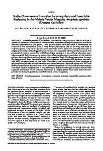
where V P0 is the P-wave vertical velocity and δ (1,2) are the anisotropic coefficients defined in Appendix C. Before giving the corresponding expressions for shear waves, it is necessary to review some relevant polarization properties of S-waves for orthorhombic anisotropy. A drawing of typical phase-velocity sheets in orthorhombic media is shown in Figure 1. The outer (P-wave) phase-velocity surface is usually separated from the two sheets corresponding to split shear waves. The shear-wave phase velocities in orthorhombic media

¤2

(P)

− t0

.

(11)

Although this approach looks relatively straightforward, application of equation (11) is compounded by the fact that only one (PSV) converted wave can be generated in each symmetry plane; this will be discussed in more detail below. NMO VELOCITIES OF P- AND S-WAVES IN AN ORTHORHOMBIC LAYER

Having obtained the relationships between the NMO ellipses of pure and converted modes in orthorhombic media, we next need to discuss the dependence of NMO velocities

FIG. 1. Sketch of body-wave phasepvelocity surfaces in orthorhombic media. The value ai j = ci j /ρ, where ci j are the elastic stiffness coefficients and ρ is the density.

150

Grechka et al.

coincide in certain directions corresponding to the so-called point singularities (Crampin and Yedlin, 1981), such as point A in Figure 1. We assume that the singularities are far enough from vertical so that the fast shear wave, S1 , can be distinguished from the slow wave, S2 , in some vicinity of the vertical direction sufficiently large to obtain NMO velocities. While applying the equivalence with VTI media to S-waves, we must remember that the polarization of shear waves with respect to the vertical incidence plane varies with azimuth. Suppose the fast vertically traveling shear wave S1 is polarized in the x2 -direction and, therefore, represents a pure transverse (SH) wave for any phase direction in the [x1 , x3 ] plane. As we move along the phase-velocity surface of the S1 -wave around the x3 -axis to the [x2 , x3 ] plane (Figure 1), its polarization changes from transverse (cross-plane) to in-plane (in other words, from SH in the [x1 , x3 ] plane to SV in the [x2 , x3 ] plane). Thus, according to the kinematic analogy with vertical transverse isotropy, the S1 -wave propagating in the [x1 , x3 ] plane is equivalent to the SH-wave in VTI media, while in the [x2 , x3 ] plane it is equivalent to the SV-wave. Likewise, the polarization of the S2 -wave changes from SV in the [x1 , x3 ] plane to S H in the [x2 , x3 ] plane. This property of S-waves has a direct bearing on the form of their NMO velocities listed below (again, the superscript 1 corresponds to the [x2 , x3 ] plane and 2 corresponds to the [x1 , x3 ] plane):

(1) 1 ,nmo

p √ 1 + 2 γ (2) = c66 /ρ, p = VS1 1 + 2 σ (1) ,

(14)

(2) 2 ,nmo

= VS2

p 1 + 2 σ (2) , p √ = VS2 1 + 2 γ (1) = c66 /ρ,

(15)

(2) 1 ,nmo

VS VS and

VS

(1) 2 ,nmo

VS

= VS1

where

à σ

(2)

= Ã

σ (1) =

V P0 VS2 V P0 VS1

!2 !2

¡

¢ ² (2) − δ (2) ,

¡

² (1) − δ

(16)

¢ (1)

.

The anisotropic coefficients ² ( j) and γ ( j) are described in Appendix C. The vertical shear velocities VS1 and VS2 (we assume VS1 > VS2 ) in equations (14)–(16) are related to Tsvankin’s (1997) vertical velocity VS0 (Appendix C) as

s

VS2 = VS0 ,

VS1 = VS0

1 + 2γ (1) . 1 + 2γ (2)

(17)

Equations (11) and (13)–(16) provide an analytic basis for obtaining the parameters of an orthorhombic layer from moveout measurements. Note that the NMO velocities of three pure modes depend on eight (out of nine) parameters of the orthorhombic layer. The only coefficient that makes no contribution to the NMO velocities is δ (3) (or c12 ); this parameter is defined in the horizontal symmetry plane and cannot be found from near-vertical measurements of NMO velocity. Another important observation relates to the fact that the SH-wave ve-

locities in the symmetry planes [equations (14) and (15)] are identical: (2) 1 ,nmo

VS

(1) . 2 ,nmo

= VS

(18)

This indicates a possible redundancy in the moveout measurements that can be used to increase the accuracy of the inversion procedure. Suppose we have found the zero-offset traveltimes of all three pure modes (P, S1 , S2 ) and their NMO velocities in the symmetry planes (in our case, using P- and PS-waves). Since the ratios of the vertical velocities can be obtained from the zero-offset traveltimes, only one vertical velocity must be determined. Therefore, for a total of seven unknowns (V P0 , ² (1,2) , δ (1,2) , γ (1,2) ), there are only six moveout equations (13)–(15). Separating out the SH-wave equations that depend on γ (1,2) (or a single stiffness coefficient, c66 ), we have four moveout equations for P- and SV-waves that include five unknown parameters (V P0 , ² (1,2) , δ (1,2) ). Clearly, the number of unknowns exceeds the number of equations by one, and the inversion is impossible without including some additional information. The same underdetermined inverse problem, as discussed in detail by Tsvankin and Thomsen (1995), arises for vertical transverse isotropy (or, equivalently, in each vertical symmetry plane of orthorhombic media). To resolve the anisotropic coefficients, we assume that the layer thickness is known and all vertical velocities can be found from the zero-offset traveltimes. Possible alternatives include use of dipping events or long-spread (nonhyperbolic) moveout, but this information was not available in our physical modeling experiment. In the discussion above, we assumed that the combination of P- and PS-waves is sufficient to determine the symmetryplane NMO velocities for all three pure modes. Polarization properties of shear waves, however, have serious implications for the generation of the converted modes used in our algorithm. Since the phase-velocity sheets (and the corresponding wavefronts) of the waves P, S1 , and S2 are continuous, from the kinematic viewpoint the converted waves PS1 and PS2 can be recorded in all azimuthal directions. However, P-waves propagating in either vertical symmetry plane of a horizontal orthorhombic layer cannot generate the converted PSHwave because the particle motion should be confined to the incidence plane. Thus, the PS1 -wave does not exist in the [x1 , x3 ] plane, while the PS2 -wave cannot be excited in the [x2 , x3 ] plane. Moreover, PSH-type reflections will also be weak near those symmetry planes because shear-wave polarizations change in a continuous fashion. However, the NMO velocities of these (in practice unmeasurable) converted waves in the symmetry planes can be reconstructed from moveout measurements in other azimuthal directions by taking advantage of the known (elliptical) azimuthal dependence of the NMO-velocity function. INVERSION OF PHYSICAL MODELING DATA

Scaled physical modeling over anisotropic materials has proven to be useful in testing theoretical predictions of various wave-propagation phenomena. A number of publications are devoted to simulations of fracture-induced anisotropy and measurements of shear-wave splitting (e.g., Tatham et al., 1987; Ebrom et al., 1990). In a series of experiments with

P- and PS -Waves in Orthorhombic Media

orthorhombic phenolic laminate, Cheadle et al. (1991) and Brown et al. (1991) recorded transmitted waves propagating in different directions and determined the stiffness coefficients of the material. Sayers and Ebrom (1997) generated wideangle P-wave data for an orthorhombic material in vertical seismic profiling (VSP) geometry and used a nonhyperbolic moveout equation to reconstruct the P-wave group-velocity surface. Here, we simulate a reflection seismic survey over an azimuthally anisotropic layer by recording pure and converted reflected waves generated in a rectangular block of orthorhombic Phenolite XX-324. Previous experiments with the same material are described by Gibson and Theophanis (1996). Laboratory setup The model for the ultrasonic experiment was constructed of six 30.0 × 5.0 × 14.81-cm blocks of Phenolite XX-324, a composite material with orthorhombic symmetry. The slow (in terms of P-wave velocity) axes of the blocks were aligned in a direction that will be called the x1 -axis of the model. The blocks were bonded with epoxy to make a sample with dimensions 30.0 × 30.0 × 14.81 cm (z = 14.81 cm is the vertical thickness). The epoxy bonding of the joints was performed under a uniform pressure of 15 psi. The reflection coefficient for the epoxy joints between layers was tested with both Pand S-waves of the appropriate frequencies and found to be unmeasureably small. Taking into account the seismic velocities and size of the Phenolite model, ultrasonic transducers were chosen to produce an acoustic wavelength close to one-sixth of the model thickness. This wavelength corresponds to frequencies of approximately 100 kHz for S-waves and 200 kHz for P-waves. Vertical and horizontal contact transducers (supplied by Panametrics, Waltham, MA), used as source and receiver, had a diameter of 1.0 inch. The central frequency and bandwidth of the transducers can be adjusted by varying the width of the excitation pulse. The pulse was produced by a Hewlett Packard 214B high-voltage pulse generator (it has independent control of voltage, pulse width, and repetition rate). Data were collected directly from the receiving transducer with a Lecroy 9304A oscilloscope, which has real-time signal-averaging capability for noise reduction as well as a disk drive for data storage. CMP surveys were simulated by recording arrivals reflected from the bottom of the block (free surface). Gathers were acquired along differently oriented CMP lines, with offsets for each line ranging from 5 to 25 cm with 2-cm increments. Data were collected sequentially with P–P transducer pairs at azimuths 0◦ , 45◦ , 90◦ , and 135◦ with respect to axis x1 and with P–S transducer pairs along azimuths 0◦ , 30◦ , 60◦ , and 90◦ . Processing P-wave data We begin with processing reflection data recorded by vertical transducers along azimuths 0◦ , 45◦ , 90◦ , and 135◦ (Figure 2). The seismogram for azimuth 135◦ is not shown in Figure 2 because it looks similar to that for azimuth 45◦ . The most prominent feature of the seismograms is a significant azimuthal variation in the P-wave traveltimes. Clearly, the moveout velocity increases as the azimuth changes from 0◦ to 90◦ , which leads to a corresponding decrease in the P-wave traveltime for any fixed offset. To reconstruct the azimuthal dependence

151

of moveout velocity, we performed conventional hyperbolic semblance analysis and displayed the results in the semblance panels (Figure 2d–f). (We used a nonlinear amplitude scale to enhance semblance maxima and muted out all semblance values below a certain level.) The position of the semblance maximum on the velocity axis varies with azimuth by more than 1.0 km/s (42%), indicating a high degree of P-wave azimuthal anisotropy. Having picked the moveout velocities from the semblance panels, we calculated the corresponding hyperbolic moveout curves for each azimuth and superimposed them on the seismograms (dashed lines). Since the zero-offset traveltimes of the semblance maxima are larger than the times of the first breaks, we introduced an appropriate correction in the picked t0 that allowed us to match the actual arrival times on the seismograms. Clearly, except for relatively small deviations at the very far offsets, the hyperbolic moveout approximation is close to the traveltimes in all azimuthal directions. Therefore, nonhyperbolic moveout on the spreads used in the experiment (the maximum offset-to-depth ratio is 1.7) is relatively weak for the Phenolite model (for more details, see “Discussion”). Using the P-wave moveout velocities measured in all four azimuthal directions, we reconstructed the P-wave NMO ellipse (Figure 3). The data points, which correspond to finite-spread moveout velocities, lie very close to the best-fit elliptical curve (the maximum deviation is 1.6% at azimuth 90◦ ). This serves as another corroboration of the small magnitude of nonhyperbolic moveout and high accuracy of the hyperbolic moveout equation parameterized by the analytic NMO velocity. The azimuths of the axes of the best-fit NMO ellipse in the coordinate frame of our experiment are 0.6◦ and 90.6◦ . As discussed above, in orthorhombic media these axes should be aligned with the vertical symmetry planes; indeed, our results are in good agreement with the expected symmetry-plane orientation. The values of the NMO velocities along the axes (i.e., in the symmetry planes; see Table 1) were combined with the vertical velocity (P) VP0 = 2z/t0 = 3.57 km/s to compute the anisotropic param(1,2) eters δ from equations (13) (δ (1) = 0.073, δ (2) = −0.22). No other information can be obtained from P-wave moveout measurements for a horizontal reflector on conventional-length spreads. Processing converted-wave data To obtain moveout velocities of converted waves, we processed seismograms recorded by horizontal transducers oriented along four CMP lines at azimuths 0◦ , 30◦ , 60◦ , and 90◦ (Figures 4 and 5). Although P-waves can be seen on all four sections of horizontal displacement, the largest semblance Table 1. NMO velocities (in km/s) in the symmetry planes of the model. The velocities of the P- and PS-waves were obtained from the reconstructed NMO ellipses; the velocities of the pure shear reflections were computed using equation (11). Azimuth Reflection PP P S1 P S2 S1 S1 S2 S2

0◦ 2.68 1.92 2.10 1.36 1.83

90◦ 3.82 2.84 2.33 2.14 1.35

152

Grechka et al.

maximum corresponds to the second arrival, which we identified as a converted wave. Our interpretation is based on the zero-offset traveltimes of these modes, their relatively low moveout velocities, and predominantly horizontal polarization. Since the wavefield was excited by a vertical source, we did not expect to record strong pure shear reflections at the moderate offsets used in the experiment. Although S1 S1 - and S2 S2 -waves can be seen on the horizontal displacement component, their semblance maxima are not focused enough for accurate velocity picking. Therefore, for each section we determined the moveout velocity of a single (PS) mode corresponding to the most pronounced semblance maximum and used it in moveout inversion. After obtaining the model parameters, we computed the reflection moveout of pure S-waves and plotted it against the actual arrivals to verify the accuracy of our algorithm.

It is clear from both the seismograms and semblance panels that we observe two different converted waves, each one dominating the radial component of the wavefield in a certain range of azimuthal angles. While the second arrival at azimuths 0◦ and 30◦ (Figure 4) has a zero-offset traveltime of 0.148 ms, the value of t0 for the second arrival at 60◦ and 90◦ (Figure 5) is noticeably smaller (0.119 ms). The difference in the zerooffset traveltimes allows us to identify the PS reflection in Figure 4 as the slow converted wave (PS2 ) and the corresponding event in Figure 5 as the fast wave (PS1 ). The magnitude of shear-wave splitting in the vertical direction is sufficient for the two converted waves to be well separated in time. The vertical shear-wave velocities VS2 and VS1 can be calculated from the zero-offset traveltimes and the known layer thickness using (P S ) the equation t0 i = z/VSi + z/V P0 , i = 1, 2; we obtained VS1 = 1.91 km/s and VS2 = 1.39 km/s.

FIG. 2. Seismograms of the vertical displacement component recorded at azimuths (a) 0◦ , (b) 45◦ , and (c) 90◦ and the corresponding semblance panels (d–f). Dashed lines mark P-wave moveouts picked from the semblance panels.

P- and PS -Waves in Orthorhombic Media

Figures 4 and 5 confirm our prediction that only one converted wave (close to the PSV type) can be observed in a vicinity of each symmetry plane. The fast wave PS1 has the SV polarization in the [x2 , x3 ] plane (azimuth 90◦ ) and therefore is recorded at azimuths 60◦ and 90◦ . In contrast, the sections at 0◦ and 30◦ contain an intensive PS2 arrival, with the SV polarization in the [x1 , x3 ] plane. It is likely that the arrival with the zero-offset traveltime close to 0.12 ms that can be seen at small offsets in Figure 4b is the PS1 reflection, but its amplitude is not sufficient to generate a focused semblance maximum. Even if the SH-type waves were excited at the reflecting boundary, they would not be recorded by our in-line horizontal receiver. In general, PS-wave processing in azimuthally anisotropic media requires two orthogonal horizontal geophones (in-line and cross-line) that would record the horizontal displacement of both split converted modes. Then the in-line and cross-line seismograms should be simultaneously rotated to separate the converted arrivals; this algorithm in application to pure SS reflections excited by a single source is described in detail by Thomsen (1988). Because of the high degree of S-wave splitting in our model, the converted waves were separated in time at all offsets and the rotation was unnecessary. A cross-line receiver, however, could have helped to enhance the converted waves with quasi-SH polarization near the vertical symmetry planes. Using the semblance maximum of the most intensive arrival (Figures 4c,d and 5c,d), we obtained the NMO velocities of each converted wave in two azimuthal directions and plotted the corresponding moveouts with dashed lines in Figures 4a,b and 5a,b. As was the case with P-waves, the best-fit hyperbolic moveout curve is close to the PS traveltimes, with deviations becoming noticeable only at far offsets. Most importantly, the velocities corresponding to the semblance maxima for each converted wave exhibit a pronounced azimuthal dependence. For instance, there is a significant increase in the best-fit move-

FIG. 3. Moveout velocities corresponding to the semblance maxima for the reflected P-wave (dots) and the best-fit NMO ellipse (solid line).

153

out velocity of the PS1 reflection from an azimuth of 60◦ to 90◦ . In general, a minimum of three different azimuthal moveout measurements is necessary to recover the NMO velocity for each mode. However, since the orientation of the NMO ellipses (i.e., the azimuths of the symmetry planes) has already been determined from P-wave data (Figure 3), two sufficiently separated azimuths provide enough information to find the values of the elliptical semi-axes. [Note: If the medium does not have vertical symmetry planes (e.g., the symmetry is lower than orthorhombic), the NMO ellipses of pure and converted modes may have different orientations.] The NMO velocities of both converted waves, reconstructed from the data, are shown in Figure 6. The least trivial part of the converted-wave processing is determination of the moveout velocities of the physically nonexistent reflected PSH-waves in the symmetry planes (PS1 in the [x1 , x3 ]-plane and PS2 in the [x2 , x3 ]-plane). These velocities have been obtained essentially by extrapolating the moveout measurements of the waves PS1 and PS2 in other azimuthal directions using the known functional form of the azimuthal dependence of NMO velocity. Estimation of anisotropic parameters Substituting the symmetry-plane NMO velocities of the converted waves into equation (11), we computed the corresponding velocities of the pure shear modes (Table 1) and plotted their NMO ellipses with dashed lines in Figure 6. Although the time delay between the vertically traveling shear and converted waves is rather significant, the NMO ellipses of the S-waves (as well as the ellipses of the converted waves) intersect each other as a result of the influence of the anisotropic coefficients in equations (14) and (15). Since the vertical velocities and coefficients δ (1,2) are already known, equations (14)–(16) make it possible to find anisotropic parameters ² (1,2) and γ (1,2) from the symmetry-plane NMO velocities of the pure shear waves. The set of Tsvankin’s (1997) parameters (Appendix C) of the Phenolite model obtained from the moveout inversion is as follows:

V P0 = 3.57 km/s,

VS0 = 1.91 km/s,

δ (2) = −0.22,

δ (1) = 0.073,

² (2) = −0.16,

² (1) = 0.11,

γ (2) = −0.25,

γ (1) = −0.028.

The difference between the coefficients δ (1) and δ (2) is responsible for the azimuthal variation in the P-wave NMO velocity, while ² (1) − ² (2) determines the variation in the P-wave horizontal velocity between the x2 - and x1 -axes. The values γ (1) and γ (2) define the velocity anisotropy of the SH-waves in the symmetry planes (S1 in the [x1 , x3 ] plane and S2 in the [x2 , x3 ] plane). The only anisotropic coefficient not determined from moveout inversion is δ (3) . As mentioned earlier, this parameter has no influence on either the vertical velocities or the NMO velocities of any mode and therefore is not constrained by conventional-spread reflections from horizontal interfaces. The coefficient δ (3) , however, does contribute to the traveltime

154

Grechka et al.

of the direct P-wave arrival in the horizontal plane that can be identified at relatively large offsets in Figures 4a,b and 5a,b. Like the other δ coefficients, δ (3) influences the phase velocities only away from the coordinate directions of the orthorhombic model. Therefore, we estimated δ (3) from the group velocity of the direct P-wave arrival at azimuths 30◦ and 60◦ (Figure 7). We found that the value of δ (3) = −0.21 gives the best fit to the group-velocity measurements in both azimuthal directions. Thus, we have obtained the full set of Tsvankin’s parameters for the Phenolite model. Using the expressions for these parameters in terms of the stiffness coefficients ci j (Appendix C),

we calculated the following stiffness matrix (in km2 /s2 ):



8.58 2.74   2.01 ci j =  0 ρ    0 0

2.74 15.51 9.76 0 0 0

2.01 9.76 12.74 0 0 0

0 0 0 3.65 0 0

0 0 0 0 1.93 0

 0 0    0  . 0    0  1.84 (19)

FIG. 4. Seismograms of the horizontal in-line displacement component recorded at azimuths (a) 0◦ and (b) 30◦ and the corresponding semblance panels (c,d). Dashed lines mark PS2 -wave moveouts picked from the semblance panels. Moveouts of the pure P- and S2 -wave reflections, computed using the inversion results, are marked by dots.

P- and PS -Waves in Orthorhombic Media

Verification of inversion results There are several ways to check the accuracy of the inversion algorithm. First, as discussed above, we have some redundancy in the moveout measurements since the NMO velocity of the fast mode S1 S1 at azimuth 0◦ ([x1 , x3 ] plane) should be equal to the S2 S2 -wave NMO velocity at azimuth 90◦ [see equation (18)]. These velocities correspond to the S H -waves in the symmetry planes and therefore could not be measured from the data directly because of the absence of PSH reflections. Nevertheless, the values computed using the extrapolated NMO ellipses of both converted waves are remarkably close to each other (Table 1).

155

Another way of verifying the inversion results is to compute the traveltimes of reflection arrivals not used for parameter estimation and check the extent to which the predicted moveouts match the data. PP-wave moveout curves calculated for the obtained model parameters are shown in Figures 4b and 5a (azimuths 30◦ and 60◦ ). Although the P-wave NMO ellipse was built from moveout data at azimuths 0◦ , 45◦ , 90◦ , and 135◦ , it accurately predicts P-wave moveout in these intermediate directions. In addition, we computed the traveltimes of both pure shear reflections, which are excited by the source together with P-waves and essentially represent a byproduct of the experiment. Figures 4a,b and 5a,b show that the predicted moveout

FIG. 5. Seismograms of the horizontal in-line displacement component recorded at azimuths (a) 60◦ and (b) 90◦ and the corresponding semblance panels (c,d). Dashed lines mark PS1 -wave moveouts picked from the semblance panels. Moveouts of the pure P- and S1 -wave reflections, computed using the inversion results, are marked by dots.

156

Grechka et al.

curves lie close to these relatively weak shear-wave arrivals not used in the inversion. The most direct check of the inversion procedure is a comparison between the predicted and measured group velocities in certain directions. The reflection data used in our experiment illuminate a limited range of group (ray) angles with respect to vertical, and the maximum incidence angle for pure reflections reaches about 40◦ . Still, the shear-wave inversion allowed us to obtain coefficients ² (1) and ² (2) responsible for √ the √ P-wave horizontal velocity along the axes x1 ( c11 /ρ) and x2 ( c22 /ρ). These results are in excellent agreement with the direct measurements of the P-wave horizontal velocities given in Table 2. Also, the NMO velocities of the SH-waves in the symmetry planes √ should be equal to the corresponding horizontal velocity c66 /ρ [see equations (14) and (15)]. Although the moveout of the SH-waves was estimated by extrapolating the NMO ellipses of the converted waves rather than from actual S H -reflections, the inverted SH-wave horizontal velocity is also close to the directly measured value. There was no need to check the horizontal velocities of the SV-waves in each vertical symmetry plane because they are equal to the corresponding vertical velocities. We conclude that the underlying assumption about the orthorhombic symmetry of the model is valid, and the accuracy

Table 2. Comparison of the horizontal velocities obtained from moveout inversion with the directly measured values.

√ √c11 /ρ √c22 /ρ c66 /ρ

Inverted velocity (km/s)

Measured velocity (km/s)

Difference (%)

2.93 3.94 1.36

2.92 4.02 1.39

0.2 −1.9 −2.6

FIG. 6. The converted-wave NMO ellipses (solid lines) reconstructed from the picked moveout velocities (dots) and the NMO ellipses of pure shear reflections (dashed) computed from the NMO velocities of P- and PS-waves.

of the moveout inversion is sufficient for obtaining the orientation of the symmetry planes and the elastic parameters of the medium. DISCUSSION

Despite the excellent results of the inversion procedure, the model used in our experiment was relatively simple (a single layer) and strongly anisotropic, which helped separate the split converted waves in a straightforward fashion. Below, we discuss the main potential problems in the application of this algorithm to processing of multicomponent data acquired over typical vertically inhomogeneous fractured formations. Nonhyperbolic moveout.—Our inversion scheme operates with NMO velocities obtained from the data using the hyperbolic approximation for reflection traveltimes. One may believe that for converted waves this approximation is inherently contradictory because PS-wave moveout is known to be nonhyperbolic, even in a homogeneous isotropic medium. However, as shown by Tsvankin and Thomsen (1994) for vertical transverse isotropy, PS moveout curves typically do not deviate much from a hyperbola on conventional-length spreads (i.e., close to the reflector depth), especially for positive values of the anisotropic parameter σ . This conclusion remains entirely valid in the symmetry planes of orthorhombic media if we use the appropriate σ coefficient [equation (16)]. Both σ (1) and σ (2) were positive (and small) in our physical modeling

FIG. 7. The seismograms of the horizontal displacement component at azimuths 30◦ and 60◦ . The straight dashed lines mark the direct P-wave arrival. The group velocities determined from the slopes of the dashed lines are 2.860 km/s (30◦ ) and 3.200 km/s (60◦ ).

P- and PS -Waves in Orthorhombic Media

experiment, and nonhyperbolic moveout for PS arrivals was not significant, despite a relatively large offset-to-depth ratio of 1.7. The magnitude of nonhyperbolic moveout for P-waves mostly depends on the degree of anellipticity of the model measured by the parameters (Tsvankin, 1997) η(i) =

² (i) − δ (i) , 1 + 2δ (i)

(i = 1, 2).

Neither η(1) nor η(2) exceeded 10% in our model (η(1) = 0.042, η(2) = 0.098), and P-wave moveout on the spreadlengths used in the experiment was close to hyperbolic as well. Another factor that helped mitigate the influence of nonhyperbolic moveout for both P- and PS-waves is a rapid decrease of the amplitudes with offset (Figures 4a,b and 5a,b), most likely caused by the source radiation pattern. In realistic layered media, the magnitude of nonhyperbolic moveout may be enhanced by vertical inhomogeneity. In this case, stable recovery of NMO velocities requires either muting out offsets exceeding the reflector depth (as is conventionally done in seismic processing) or applying nonhyperbolic semblance analysis based, for instance, on the equation developed by Tsvankin and Thomsen (1994). Strength of azimuthal anisotropy and shear-wave splitting.— In the inversion for the medium parameters, we used the zerooffset traveltimes and azimuthally dependent NMO velocities of the converted waves PS1 and PS2 . These measurements require prior separation of the split converted waves on the seismograms. The strength of shear-wave splitting near vertical can be described by the shear-wave splitting parameter γ (S) , which is close to the fractional difference between the shear-wave vertical velocities [γ (S) = (VS2 /VS22 − 1)/2 ≈ (VS1 /VS2 − 1)]. For 1 the Phenolite sample, the splitting coefficient turned out to be uncommonly large (γ (S) = 0.44), and the PS1 and PS2 arrivals were well separated at all offsets used in the experiment. If γ (S) were smaller, the converted waves would interfere near vertical, making the moveout velocities much more difficult to obtain. In this case, it is necessary to deploy two horizontal geophones and use a rotation algorithm (Thomsen, 1988) to separate orthogonally polarized split converted waves. This operation may reduce the accuracy of moveout inversion even in a single layer. The situation becomes much more complicated in stratified media, especially if the target layer is overlain by an azimuthally anisotropic overburden. In principle, equations (6)–(8) can be used to obtain the effective and interval NMO ellipses of pure shear modes from those of P- and PS-waves. However, the data may be too corrupted by multiple splitting in the overburden for reliable identification of the converted waves. Shear-wave point singularities.—The problem of shear-wave singularities is directly related to the issue of the magnitude of shear-wave splitting discussed above. We assumed that the phase-velocity (or slowness) sheets of waves S1 and S2 do not intersect in some vicinity of the vertical direction. In other words, shear-wave point singularities (point A in Figure 1), which always exist in orthorhombic media, are supposed to be sufficiently far from vertical. The position of singularities with respect to the vertical axis is determined by the value of

157

the parameter γ (S) : the separation of the shear-wave velocity sheets near vertical increases with γ (S) , and singularities move closer to the horizontal plane. Because of the large value of γ (S) in the Phenolite model, the singularity closest to the vertical axis corresponds to a phase angle (with respect to vertical) of 68.5◦ . Clearly, the assumption that the phase-velocity sheets of split S-waves intersect far from vertical is satisfied. However, if γ (S) were smaller and the reflected rays for a certain range of offsets and azimuthal angles crossed a singularity region, we would record complicated converted wavefields (including multiple arrivals) that would be difficult to separate into distinct PS1 and PS2 reflections (Crampin and Yedlin, 1981; Grechka and Obolentseva, 1993). Polarization of shear waves.—The physical modeling confirmed our theoretical prediction that each of the converted waves does not exist in a vicinity of one of the symmetry planes, where its polarization becomes close to that of an SHwave (Figure 1). This fact imposes additional requirements on the number of azimuthal measurements needed to reconstruct the NMO ellipses. While three well-separated CMP lines are generally sufficient to obtain P-wave NMO ellipses (Grechka and Tsvankin, 1998), there is no guarantee that both PS reflections will be intensive enough along at least two of those lines. (We need two or more measurements of the NMO velocity for each PS-wave to build the NMO ellipse, assuming that the symmetry-plane orientation has been determined from P-wave data.) We believe that acquisition of converted-wave data along four well-separated CMP lines (and on two horizontal displacement components) should be accepted as a minimum requirement. Useful redundancy in PS moveout measurements can be provided by 3-D surveys with a wide range of source-receiver azimuths. Sorting into common conversion point gathers.—One of the essential steps in processing of mode-converted reflections is sorting the data into common conversion point gathers. If the medium is laterally heterogeneous, the offset dependence of the reflection (conversion) point of PS-wave arrivals on CMP gathers may cause distortions in velocity analysis and degrade the quality of stack. Both our theoretical and physical models, however, were horizontally homogeneous, so common conversion point sorting was unnecessary. In principle, the moveoutinversion procedure introduced here can be performed on either CMP or common conversion point gathers, but in fielddata applications it is preferable to carry out common conversion point sorting before velocity estimation. Unfortunately, the position of the conversion point in orthorhombic media depends on the anisotropic parameters, which are seldom known in advance. Therefore, azimuthal velocity analysis and moveout inversion can be carried out first on CMP gathers to obtain an approximate anisotropic model. Then these parameterestimation results can be used to sort the data into CCP gathers and to refine the model by repeating the inversion procedure. These complications show that the problem of joint inversion of P and PS traveltime data in azimuthally anisotropic media may become much more involved under less favorable circumstances than in our experiment, especially in the presence of vertical inhomogeneity. Also, a strong assumption of our method, which may not be satisfied in some subsurface

158

Grechka et al.

models, is the possibility to record P and PS reflections from the same interface. Depending on the contrasts in the elastic parameters across the reflector and the properties (e.g., the Q-factor) of the overburden, the amplitude of either the Por PS-wave may be too small for reliable application of the moveout inversion. CONCLUSIONS

We derived a moveout equation for mode-converted waves in horizontally layered anisotropic media with a horizontal symmetry plane by generalizing the approach developed for pure modes by Grechka and Tsvankin (1998). As a result of the mirror symmetry with respect to the reflectors, the traveltime series for converted waves contains only even terms in offset and, for conventional spreadlengths, reduces to a hyperbolic equation parameterized by NMO velocity. Furthermore, the azimuthal dependence of converted-wave NMO velocity has the same (elliptical) form as for pure modes and can be reconstructed from three or more moveout measurements in different azimuthal directions. The parameters of the NMO ellipse for converted waves were expressed through those of the corresponding pure modes using the generalized Dix equation of Grechka et al. (1997). This Dix-type relationship makes it possible to obtain both effective and interval shear-wave NMO velocity from the azimuthally dependent moveout of P- and PS-waves. Then interval NMO velocities of pure P and S reflections can be inverted for a subset of the anisotropic parameters that depends on the anisotropic symmetry and available wavetypes. We implemented this algorithm for orthorhombic models (typical for fractured reservoirs), taking advantage of the simplicity of moveout equations in Tsvankin’s (1997) notation. The method was tested on physical modeling data acquired over a block of azimuthally anisotropic Phenolic material known to have orthorhombic symmetry. By combining NMO velocities and zero-offset traveltimes of P- and two split PS-waves, we determined the orientation of the vertical symmetry planes and eight (out of nine) elastic parameters of the material. In the inversion procedure we used the known layer thickness to obtain the vertical velocities that otherwise would not be constrained by the reflection data. (If reflector depths are unknown, parameter estimation in orthorhombic media cannot be based solely on NMO velocities from horizontal reflectors and should include either nonhyperbolic moveout or dip dependence of NMO velocity.) The theory even allowed us to reconstruct the moveout velocities of the converted PSH-waves in the symmetry planes, although these arrivals cannot be physically excited in our model. The only elastic coefficient that could not be recovered from moveout data [δ (3) in Tsvankin’s (1997) notation] was evaluated using the group velocity of the direct P-wave. The high accuracy of the inversion procedure was verified in several ways, including a comparison of the inverted and directly measured horizontal velocities of pure modes. Although the physical modeling experiment was performed for a single orthorhombic layer, the theory remains valid for more complicated vertically inhomogeneous azimuthally anisotropic models. The main problem in the practical implementation of this algorithm is the recovery of reflection moveout of converted waves in the presence of multiple splitting in azimuthally anisotropic layers. Also, the transition from NMO

velocities of horizontal events to the anisotropic coefficients requires knowledge of vertical velocity or reflector depth. ACKNOWLEDGMENTS

We are grateful to Gilein Steensma (CSM) and members of the A(nisotropy)-Team of the Center for Wave Phenomena at CSM for helpful discussions. We also thank Jim Brown (PGS), Jim Gaiser (Western), Ken Larner (CSM), and Reinaldo Michelena (Intevep) for their thorough reviews of the manuscript. The support for this work was provided by the members of the Consortium Project on Seismic Inverse Methods for Complex Structures at the Center for Wave Phenomena and by the U.S. Dept. of Energy (Velocity Analysis, Parameter Estimation, and Constraints on Lithology for Transversely Isotropic Sediments project within the framework of the Advanced Computational Technology Initiative). REFERENCES Brown, R. J., Lawton, D. C., and Cheadle, S. P., 1991, Scaled physical modelling of anisotropic wave propagation: Multioffset profiles over an orthorhombic medium: Geophys. J. Internat., 107, 693– 702. Cheadle, S. P., Brown, R. J., and Lawton, D. C., 1991, Orthorhombic anisotropy: A physical seismic modeling study: Geophysics, 56, 1603–1613. Corrigan, D., Withers, R., Darnall, J., Skopinski, T., 1996, Fracture mapping from azimuthal velocity analysis using 3D surface seismic data: 66th Ann. Internat. Mtg., Soc. Expl. Geophys., Expanded Abstracts, 1834–1837. Crampin, S., and Yedlin, M., 1981, Shear-wave singularities of wave propagation in anisotropic media: J. Geophys., 49, 43–46. Ebrom, D. A., Tatham, R. H., Sekharan, K. K., McDonald, J. A., and Gardner, G. H. F., 1990, Hyperbolic traveltime analysis of first arrivals in an azimuthally anisotropic medium: A physical modeling study: Geophysics, 55, 185–191. Gibson, R. L., Jr., and Theophanis, S., 1996, Ultrasonic and numerical modeling of reflections from azimuthally anisotropic media: 66th Ann. Internat. Mtg., Soc. Expl. Geophys., Expanded Abstracts, 1025–1028. Grechka, V., and Obolentseva, I., 1993, Geometrical structure of shear wave surfaces near singularity directions in anisotropic media: Geophys. J. Internat., 115, 609–616. Grechka, V., and Tsvankin, I., 1997, Moveout velocity analysis and parameter estimation for orthorhombic media: 67th Ann. Internat. Mtg., Soc. Expl. Geophys., Expanded Abstracts, 1226–1229. ——— 1998, 3-D description of normal moveout in anisotropic inhomogeneous media: Geophysics, 63, 1079–1092. Grechka, V., Tsvankin, I., and Cohen, J. K., 1999, Generalized Dix equation and analytic treatment of normal-moveout velocity for anisotropic media: Geophys. Prosp., 47, no. 2 (in print). Hubral, P., and Krey, T., 1980, Interval velocities from seismic reflection measurements: Soc. Expl. Geophys. Lynn, H., Simon, K., Bates, C., and Van Doc, R., 1996, Azimuthal anisotropy in P-wave 3-D (multiazimuth) data: The Leading Edge, 15, 923–928. Sayers, C. M., and Ebrom, D. A., 1997, Seismic traveltime analysis for azimuthally anisotropic media: Theory and experiment: Geophysics, 62, 1570–1582. Schoenberg, M., and Helbig, K., 1997, Orthorhombic media: Modeling elastic wave behavior in a vertically fractured earth: Geophysics, 62, 1954–1974. Seriff, A. J., and Sriram, K. P., 1991, P-SV reflection moveouts for transversely isotropic media with a vertical symmetry axis: Geophysics, 56, 1271–1274. Tatham, R. H., Matthews, M. D., Sekharan, K. K., Wade, C. J., and Liro, L. M., 1987, A physical model study of shear-wave splitting and fracture intensity: 57th Ann. Internat. Mtg., Soc. Expl. Geophys., Expanded Abstracts, 642–645. Tessmer, G., and Behle, A., 1988, Common reflection point datastacking technique for converted waves: Geophys. Prosp., 36, 671–688. Thomsen, L., 1986, Weak elastic anisotropy: Geophysics, 51, 1954– 1966. ——— 1988, Reflection seismology over azimuthally anisotropic media: Geophysics, 53, 304–313. Tsvankin, I., 1997, Anisotropic parameters and P-wave velocity for

P- and PS -Waves in Orthorhombic Media orthorhombic media: Geophysics, 62, 1292–1309. Tsvankin, I., and Thomsen, L., 1994, Nonhyperbolic reflection moveout in anisotropic media: Geophysics, 59, 1290–1304. ——— 1995, Inversion of reflection traveltimes for transverse isotropy:

159

Geophysics, 60, 1075–1107. Wild, P., and Crampin, S., 1991, The range of effects of azimuthal isotropy and EDA anisotropy in sedimentary basins: Geophys. J. Internat., 107, 513–529.

APPENDIX A NMO EQUATION FOR CONVERTED WAVES IN MEDIA WITH A HORIZONTAL SYMMETRY PLANE

Here, we derive an exact equation for NMO velocity of converted waves valid in horizontally layered media with a horizontal symmetry plane. Let us consider a converted mode of arbitrary type recorded on CMP lines with different azimuthal orientation but the same CMP location (Figure A-1). For a fixed midpoint x1 = x2 = 0, the reflection traveltime of a given mode can be represented as a function of the source coordinates {x1 , x2 } (the corresponding receiver coordinates are {−x1 , −x2 }). Following the approach of Grechka and Tsvankin (1998), we expand the two-way reflection traveltime t(x) in a double Taylor series in the vicinity of the CMP:

t(x) = t0 +

2 X

t,i xi +

i=1

¯ ∂t ¯¯ t,i ≡ ¯ ∂ xi ¯

2 1 X t,i j xi x j + · · · , 2 i, j=1

where

, x1 =x2 =0

t,i j

¯ ∂ 2 t ¯¯ ≡ ¯ ∂ xi ∂ x j ¯

(A-1)

, x1 =x2 =0

and t0 ≡ t(0) is the two-way zero-offset traveltime. In the pure-mode case, NMO velocity in CMP geometry is not influenced by reflection-point dispersal, and reflected rays can be assumed to travel from the zero-offset reflection point (Hubral and Krey, 1980). Therefore, the moveout expansion similar to equation (A-1) can be rewritten for pure modes

through the one-way traveltimes, and the spatial derivatives of t can be expressed through the horizontal components of the slowness vector (Grechka and Tsvankin, 1998). Unfortunately, this convenient simplification is not valid for converted waves because the reflection traveltime is calculated along two segments, each corresponding to different modes. Also, the offset dependence of the coordinates of the reflection point y [which lies on the reflector f (y) = 0, Figure A-1] can no longer be ignored, although this deviation does not contribute explicitly to our final NMO equation. We restrict ourselves to horizontally layered models with a horizontal symmetry plane in which the reflection traveltime of any converted mode remains the same if we interchange the source and receiver (see Appendix B). This reciprocity with respect to the source and receiver positions [t(x 1 , x2 ) = t(−x1 , −x2 )] removes another complication associated with mode conversions—the odd terms in offset contained in the traveltime equation (A-1). Keeping only the zero-offset traveltime and the quadratic term in the Taylor series expansion (A-1), we obtain the squared two-way CMP traveltime as

t 2 (x) = t02 + 4

2 X

Wi j xi x j ,

(A-2)

i, j=1

where W is a symmetric matrix of the second traveltime derivatives,

¯ t0 ∂ 2 t ¯¯ Wi j = . ¯ 4 ∂ xi ∂ x j ¯ x1 =0

(A-3)

x2 =0

The factor 1/4 makes the matrix W compatible with the corresponding matrices for pure-mode reflections defined through one-way traveltimes. Equation (A-2) represents a hyperbolic approximation of the converted-mode reflection traveltime. The source coordinates can be expressed through the half-offset h and azimuth of the CMP line α:

x1 = h cos α,

x2 = h sin α.

(A-4)

Equation (A-2) then becomes

¡ t 2 (h, α) = t02 + 4h 2 W11 cos2 α ¢ + 2W12 sin α cos α + W22 sin2 α . (A-5)

According to the definition of the NMO velocity Vnmo ,

t 2 (h, α) = t02 + FIG. A-1. Reflection-point dispersal for converted waves cannot be ignored in the derivation of NMO velocity. Also, if the overburden does not have a horizontal symmetry plane or the reflector is dipping, the minimum of the traveltime field will be shifted from the CMP location.

4 h2 2 (α) Vnmo

+ ···.

(A-6)

Combining equations (A-5) and (A-6) yields −2 Vnmo (α) = W11 cos2 α + 2 W12 sin α cos α + W22 sin2 α.

(A-7)

160

Grechka et al.

Equation (A-7) is identical to the NMO expression for pure modes given in Grechka and Tsvankin (1998), but matrix W for converted waves is expressed through two-way traveltimes. Another way to prove that the azimuthal dependence of NMO

velocity has the same functional form for pure and converted waves is described in Appendix B, which also introduces a simple relationship between the NMO velocities of converted and pure modes.

APPENDIX B RECIPROCAL PROPERTIES AND GENERALIZED DIX EQUATION FOR CONVERTED-WAVE MOVEOUT

Here, we show that the reflection traveltime of a converted wave in a plane layer with a horizontal symmetry plane is reciprocal with respect to the source and receiver positions (i.e., it remains the same when we interchange the source and receiver). The reciprocity implies the absence of odd terms in the traveltime series and helps extend the generalized Dix equation of Grechka et al. (1999) to converted waves.

Reciprocity of converted-wave traveltime Let us consider the converted PS-wave traveling along ray S RG and build a reciprocal ray G 1 R1 G, with G being in the middle of SG 1 (Figure B-1). Our goal is prove that the traveltimes along rays S RG and G 1 R1 G are equal to each other. Because of the presence of the horizontal symmetry plane, the upgoing and downgoing rays with the same values of the horizontal slowness components p1 and p2 will be symmetric with respect to the horizontal plane; also, the group velocities along these rays are equal to each other. The same symmetry holds for two downgoing rays with the horizontal slownesses of the same magnitude but opposite signs. Hence, to find the reflected PS-wave from G 1 to G, we generate a downgoing P-ray G 1 R1 (Figure B-1) with the horizontal slownesses (− p1 ) and (− p2 ), where p1 and p2 correspond to ray SR. Then G 1 R1 will represent a mirror image of SR with respect to the horizontal plane, and the traveltimes along these two rays will be identical. Also, as illustrated by the plan view in Figure B-1, the projections of R1 and R on the surface are symmetric with respect to G. Therefore, ray R1 G and the shear-wave reflected ray RG are symmetric with respect to the horizontal plane as well. In accordance with the earlier discussion of P-waves, this implies that R1 G corresponds to the ray parameters (− p1 ) and (− p2 ) and therefore represents the S-wave reflected at R1 (the horizontal slowness should be preserved during reflection/transmission). Thus, the P and S segments of the PS reflection from G 1 to G represent mirror images with respect to the horizontal plane of the corresponding segments of ray S RG. As a result, the traveltimes along S RG and G 1 R1 G coincide with each other, and the PS moveout is reciprocal with respect to the source and receiver positions.

Relationship between NMO velocities of pure and converted waves Next, we show that the NMO velocity of a converted wave in a medium with a horizontal symmetry plane can be obtained from the generalized Dix equation of Grechka et al. (1999), originally developed for pure-mode reflections. Using the PSwave in a plane layer (Figure B-1) as an example, we represent

its NMO velocity in the form of equation (A-7): (P S) [Vnmo (α)]−2 = W11

(P S)

(P S)

+ W22

(P S)

cos2 α + 2 W12 sin2 α,

sin α cos α (B-1)

(P S)

where matrix W is defined in equation (A-3). To relate W(P S) to matrices W(P) and W(S) of the pure modes, let us add a second identical layer beneath the first one and construct a PSSP reflected wave from the bottom of this artificial model (Figure B-1). Since the intermediate interface represents a symmetry plane, the refracted shear-wave ray R G¯ is a mirror image of ray RG, while the S-wave reflection G¯ R1

FIG. B-1. Geometry of rays used in proving the reciprocity of PS traveltimes in a layer with a horizontal symmetry plane. Rays S RG and G 1 R1 G (SG = GG 1 ) are two reciprocal PS rays reflected from the bottom of the layer (x3 = z). Ray SRG¯ R1 G 1 is reflected from the interface x3 = 2z below two identical layers. The inset shows the projections of points S, G, G 1 , R, and R1 onto the horizontal plane.

P- and PS -Waves in Orthorhombic Media

should coincide with RG and hit point R1 . Finally, R1 G 1 represents the refracted P-wave excited by G¯ R1 at R1 because it is a P-wave ray with the horizontal slowness components p1 and p2 , which should be preserved along the whole raypath of the PSSP wave. Hence, the PS-wave traveltime along ray SRG can be re¯ which in turn is equal to placed with the traveltime along S R G, one-half of the reflection traveltime along S R G¯ R1 G 1 . Since the offset SG = SG 1 /2, the NMO velocities for the PS-converted wave SRG and the reflected wave S R G¯ R1 G 1 are equal to each other. Kinematically, the PSSP-wave is analogous to a pure-mode reflection, so its NMO velocity is described by the quadratic form (A-7) (Grechka and Tsvankin, 1998). Therefore, the analogy between pure and converted waves developed here represents an alternative way to prove equation (A-7) obtained in a more formal way in Appendix A. The NMO velocity of the PSSP-wave can be written as

£

¤−2

(P SS P) (α) Vnmo

(P SS P)

+ 2 W12

(P SS P)

= W11

cos2 α (P SS P)

sin α cos α + W22

sin2 α.

(B-2)

161

The matrix W(P SS P) is determined by the generalized Dix equation of Grechka et al. (1999): (P SS P) £

W(P SS P)

t0

¤−1

(P) £

= 2t0

W(P)

¤−1

(S) £

+ 2t0

W(S)

¤−1

,

(B-3) (P) t0

(S) t0

where and are the one-way zero-offset traveltimes of the P- and S-waves in the layer and the matrices W(P) and W(S) describe the pure P- and S-reflections. Note that W(P) and W(S) are defined through one-way traveltimes τ within the layer (Grechka et al., 1999); for instance, (P)

Wi j

¯ ¯ 2 ∂ τ ¯ (P) = t0 . ¯ ∂ xi ∂ x j ¯ x1 =0

(B-4)

x2 =0

Since the NMO velocities of the PS- and PSSP-waves are (P SS P) (P S) equal to each other, Wi j = Wi j . Taking into account that ( P SS P) (P S) (P S) = 2t0 (t0 is the PS-wave zero-offset traveltime in t0 the layer), we finally obtain for matrix W(P S) (P S) £

t0

W(P S)

¤−1

(P) £

= t0

W(P)

¤−1

(S) £

+ t0

W(S)

¤−1

.

(B-5)

APPENDIX C TSVANKIN’S NOTATION FOR ORTHORHOMBIC MEDIA

Because of the identical form of the Christoffel equation, the kinematic signatures and plane-wave polarizations in the symmetry planes of orthorhombic media are given by the same equations as for vertical transverse isotropy. This equivalence was used by Tsvankin (1997) to introduce anisotropic parameters similar to the well-known Thomsen’s (1986) coefficients ², δ, and γ for VTI media. Expressions for these parameters in terms of the stiffness components ci j and density ρ are given below. V P0 —P-wave vertical velocity:

r

V P0 ≡

c33 . ρ

VS0 ≡

c55 . ρ

(C-2)

² (2) —the VTI parameter ² in the [x1 , x3 ] symmetry plane normal to the x2 -axis (this explains the superscript 2):

² (2) ≡

c11 − c33 . 2c33

(c13 + c55 )2 − (c33 − c55 )2 . 2c33 (c33 − c55 )

(C-4)

c66 − c44 . 2c44

(C-5)

The value γ (2) is close to the fractional difference between the S H -wave velocities in the x1 - and x3 -directions. ² (1) —the VTI parameter ² in the [x2 , x3 ] symmetry plane:

² (1) ≡

c22 − c33 . 2c33

(C-6)

δ (1) —the VTI parameter δ in the [x2 , x3 ] plane:

δ (1) ≡

(c23 + c44 )2 − (c33 − c44 )2 . 2c33 (c33 − c44 )

(C-7)

γ (1) —the VTI parameter γ in the [x2 , x3 ] plane:

(C-3)

The value ² (2) is close to the fractional difference between the P-wave velocities in the x1 - and x3 -directions. δ (2) —the VTI parameter δ in the [x1 , x3 ] plane:

δ (2) ≡

γ (2) ≡

(C-1)

VS0 —the vertical velocity of the S-wave polarized in the x 1 direction:

r

The value δ (2) is responsible for near-vertical P-wave velocity variations in the [x1 , x3 ]-plane; it also influences SV-wave velocity anisotropy. γ (2) —the VTI parameter γ in the [x1 , x3 ] plane:

γ (1) ≡

c66 − c55 . 2c55

(C-8)

δ (3) —the VTI parameter δ in the [x1 , x2 ]-plane (x1 plays the role of the symmetry axis):

δ (3) ≡

(c12 + c66 )2 − (c11 − c66 )2 . 2c11 (c11 − c66 )

(C-9)