SUBMITTED TO IEEE TIP (REVISED)
1
Joint-MAP Bayesian Tomographic Reconstruction with a Gamma-Mixture Prior Ing-Tsung Hsiao , Anand Rangarajan , and Gene Gindi∗
EDICS : 3-TOMO
Abstract We address the problem of Bayesian image reconstruction with a prior that captures the notion of a clustered intensity histogram. The problem is formulated in the framework of a joint-MAP (maximum a posteriori) estimation with the prior pdf modeled as a mixture-of-gammas density. This prior pdf has appealing properties, including positivity enforcement. The joint MAP optimization is carried out as an iterative alternating descent wherein a regularized likelihood estimate is followed by a mixture decomposition of the histogram of the current tomographic image estimate. The mixture decomposition step estimates the hyperparameters of the prior pdf. The objective functions associated with the joint MAP estimation are complicated and difficult to optimize, but we show how they may be transformed to allow for much easier optimization while preserving the fixed point of the iterations. We demonstrate the method in the context of medical emission and transmission tomography. Index Terms Tomographic reconstruction, joint-MAP estimation, gamma mixture, mixture decomposition. This work is supported under grant R01-NS32879 from NIH-NINDS, and grant CMRP-1334 from Chang Gung Memorial Hospital Research Fund (Taiwan). Asterisk indicates corresponding author. I.-T. Hsiao was with the Departments of Radiology and Electrical & Computer Engineering, SUNY Stony Brook, Stony Brook, NY 11784. He is now with the school of Medical Technology, Kwei-Shan, Tao-yuan 333, Taiwan, email:
[email protected] A. Rangarajan is with Department of Computer & Information Science and Engineering, University of Florida, Gainesville, FL 32611, email:
[email protected] G. Gindi∗ is with the Department of Radiology, SUNY Stony Brook, Stony Brook, NY 11784-8460, Tel: (631) 444-2539, Fax: (631) 444-6450, email:
[email protected]. July 24, 2002
SUBMITTED TO IEEE TIP (REVISED)
2
I. Introduction For many applications, image reconstruction from projections may be posed as a statistical estimation problem in which the object is estimated from noisy observed data. For Bayesian approaches, the data is supplemented by object information in the form of a suitable prior. The reconstruction is usually computed as a MAP (maximum a posteriori) estimate via minimization of a suitable objective function. A common form of prior information is that of spatial smoothness or piecewise spatial smoothness, perhaps supplemented by a positivity constraint. Historically, much effort has been devoted to the design of objective functions and associated algorithms to carry out such smoothness-constrained MAP estimation. In this work, we explore the use of a different type of prior information for the reconstruction problem, in which knowledge about the object appears in the form of its clustered intensity histogram. This kind of prior pdf would be applicable when the object voxels tend to cluster into few intensity ranges, i.e. the intensity histogram comprises a few peaks. For the application of medical transmission tomography considered here, this is an apt model. For example in the chest region, x-ray attenuation coefficients (the quality to be estimated) tend to cluster around values appropriate for lung, soft tissue and bone. For our other application, medical emission tomography (PET and SPECT), the assumption is good in certain body regions. For example in the brain, the radionuclide density (the quantity to be estimated) tends to cluster around values appropriate for grey matter, white matter and ventricles. This model is not limited to medical applications; see [19] for example. For this kind of information, a convenient form for the prior pdf is one of mixture models. Unlike smoothing, no voxel neighbor interactions are assumed; instead, the somewhat weaker assumption of intensity clustering is assumed, and the object is assumed to be positive. This leads to certain computational conveniences, including the easy imposition of positivity. In addition, for the joint-MAP estimation strategy discussed below, the problem of estimating hyperparameters becomes more tractable with this form of prior pdf than with a smoothing prior pdf. In Section II we discuss a joint-MAP framework within which to conveniently couch this problem, and in Section III we discuss details of our mixture-of gammas prior pdf. The
SUBMITTED TO IEEE TIP (REVISED)
3
joint-MAP strategy together with the form of the objectives associated with the prior pdf’s leads to an objective that is difficult to minimize, and in Section IV , we demonstrate the joint-MAP reconstruction in the context a series of transformations of this objective that solves these difficulties while preserving the fixed point of the objective. In Section V we present our medical imaging application to transmission and emission tomographic reconstruction. A discussion of pitfalls, extensions, and related work is presented in Section VI. II. Joint-MAP Framework We couch our development of an estimation method in terms of a joint-MAP framework, in which the unknown object along with hyperparameters of the prior pdf are jointly estimated. (For a survey of alternative full Bayesian approaches, see [1]. ) Let the object to be estimated be represented as a vector θ of N lexicographically ordered voxels {θn ; n = 1, . . . , N }. The object could be a 2-D or 3-D image, for instance, whose voxels are lexicographically ordered into a vector with N elements. In our Bayesian approach, θ is a random vector and θn a random variable, but notationally, we shall not distinguish between a random quantity and a particular instance of it. The observed, noisy data from which θ is to be estimated, is given by vector g, comprising lexicographically ordered elements {gm ; m = 1, . . . , M }. For realistic problems, M ≈ N . The details of the imaging system are contained in the likelihood function p(g|θ), and in Section V we give detailed expressions for this likelihood for our applications to tomography. (For the tomographic case, the measurement data g will correspond to the sinogram.) For our Bayesian approach, the prior pdf and hyperprior pdf are given by the pdf’s p(θ|ψ) and p(ψ), respectively, where ψ is a random vector of hyperparameters. In Section III, we supply detailed expressions for these terms for our particular use of a gamma-mixture prior. With the above definitions, the term p(θ, ψ|g) is then the joint posterior distribution on the object and hyperparameters. From Bayes’ theorem: p(θ, ψ|g) ∝ p(g|θ)p(θ|ψ)p(ψ)
(1)
where in (1) we use the fact that the data g depends on θ only. The three terms on the right side of (1) correspond to likelihood, prior pdf, and hyperprior pdf. Our MAP
SUBMITTED TO IEEE TIP (REVISED)
4
solution is then (θ ∗ , ψ ∗ ) ≡ arg max p(θ, ψ|g). θ ≥0,ψ
(2)
Our tactic is to use a joint-MAP alternating ascent procedure, updating, at iteration k, the object estimate θ while holding the most recent estimate of ψ fixed, then updating the parameters ψ given the latest estimate of θ. The development in Sections II, III and IV will bear out our choice of a joint-MAP alternating optimization procedure. With this strategy we can write the general framework of our joint-MAP procedure: θb
k
b ψ
k
b = arg max p(g|θ)p(θ|ψ θ ≥0
b = arg max p(g|θ)p(θ|ψ θ ≥0 k
k−1
k−1
b )p(ψ
k−1
)
),
(3)
k
= arg max p(g|θb )p(θb |ψ)p(ψ) ψ k
= arg max p(θb |ψ)p(ψ). ψ
(4)
To summarize notation, θ and ψ, the object and hyperparameters, are the random vectors k b k are estimates at that we seek to estimate. The fixed vector g is the data, and θb , ψ
iteration k of the joint-MAP procedure.1
By simply taking the negative logarithm of (1), (3) and (4), we can restate the problem in terms of objective functions. Bayes’ Theorem (1) becomes Φ(θ|g) = ΦL (g|θ) + ΦP (θ|ψ) + ΦHP (ψ)
(5)
where ΦL , ΦP and ΦHP are objectives corresponding to negative logarithms of the likelihood pdf, prior pdf, and hyperprior pdf, respectively, and the unsubscripted objective Φ corresponds to the posterior.2 The overall joint-MAP estimation (2) is now expressed as a minimization (θ ∗ , ψ ∗ ) = arg min [ΦL (g|θ) + ΦP (θ|ψ) + ΦHP (ψ)] θ ≥0,ψ 1
(6)
The iterations in (3) and (4) will converge to a local maximum of (2) provided certain mild assumptions
regarding the number of local maxima obtain [2]. These assumptions are satisfied except in pathological cases, and we have not observed any convergence problems in our many trials using (3) and (4). 2 We shall henceforth use th term , “likelihood”, “prior”, and “hyperprior” to refer to Φ L , ΦP and ΦHP , respectively. The associated pdf’s will be referred to as “prior pdf”, “likelihood pdf”, etc.
SUBMITTED TO IEEE TIP (REVISED)
5
and the joint-MAP alternating ascent (3) and (4) now becomes an alternating descent: θb
k
bk ψ
·
b = arg min ΦL (g|θ) + ΦP (θ|ψ θ ≥0
k−1
¸ k b = arg min ΦP (θ |ψ) + ΦHP (ψ) .
ψ
·
¸
) ,
(7) (8)
In (5)-(8), the arguments of the various objectives use the same conventions as the pdf b notation. Thus in (7), the objective ΦP (θ|ψ
b ψ
k−1
k−1
b ) ≡ − log p(θ|ψ
k−1
) is a function of θ, with
k
k serving as a parameter, but in (8), ΦP (θb |ψ) is now a function of ψ with θb serving
as a parameter.
Note that (7) is in itself a penalized-likelihood reconstruction that uses the latest estimate of the hyperparameters in the penalty, while (8) is a parameter fit to the latest estimate of the object. The diagram in Fig. 1 summarizes this interpretation of the jointMAP alternation. In the remainder of the paper, we will refer to the left and right side stages of Fig. 1 as the “reconstruction step” and “hyperparameter estimation step” respectively.
Penalized likelihood reconstruction k ^ θ
Fig. 1.
hyperparameter estimation ^k ψ
The alternating algorithm (7) and (8) can be summarized in this diagram. The left side is a
conventional penalized likelihood reconstruction using current parameter estimates derived from the right side. The right side is a parameter fit to the current object estimate.
In the ensuing development, we shall, without any loss of generality, temporarily model the hyperprior pdf p(ψ) as uniform, thus enabling us to conveniently drop the term Φ HP in the derivations in Sections III and IV. In Sec.VI, we discuss the incorporation of hyperpriors.
SUBMITTED TO IEEE TIP (REVISED)
6
III. Gamma-Mixture Prior With the uniform hyperprior, the right side of the alternation (8) becomes a maximum k likelihood (ML) parameter fit of ψ to θb . Our gamma-mixture prior pdf will capture
the notions of positivity and intensity clustering previously mentioned, but as a useful
preliminary step, we first introduce an independent gamma prior pdf at each voxel. This prior pdf is independent, but not identically distributed, at each voxel, and preserves positivity. This provisional prior pdf model (not our final choice!) is given by b b p(θ|ψ) = p(θ|α, β) =
N Y
n=1
p(θbn |αn , βn )
(9)
where the univariate probability is a gamma prior pdf [3] and is given by α 1 α−1 −(α/β)x p(x|α, β) = ( )α x e . β Γ(α)
(10)
This prior pdf is introduced provisionally, because its inadequacies (despite its desireable properties) will motivate the introduction of the mixture-of-gammas prior pdf that is a focus of this paper. In Sec. IV, we will show an interesting relation of our mixture-ofgammas prior pdf to (9). We note (again) in (9) that we do not distinguish between a random variable and its instance. In (9), ψ now comprises two vectors α ({αn ; n = 1, . . . , N }) and β ({βn ; n = 1, . . . , N }) which, in turn, parameterize the gamma density in (10) at each location n.
The gamma density (10) is defined [3] only for x > 0. In (10), β > 0 is the mean and β 2 /α
the variance. We assume α > 1, in which case the unique mode is given by β(1 − 1/α).
This form of prior pdf will attract the value of each voxel θbn to its local mode βn (1 − 1/αn ) √ with a relative “strength” given by the inverse standard deviation (βn / αn )−1 . Note that, like other positivity preserving asymmetric prior pdfs, the gamma prior pdf will introduce a slight bias due to the difference between mean and mode. The independent gamma prior pdf was proposed for use in emission tomography in [4]. It is convex, and preserves positivity, but impractical for our purposes. The impracticality stems from the fact that we need estimate 2N parameters (N θn ’s and N βn ’s) from M ≈ N measurements, thus leading to an overfitting problem. If, however, the object θ comprises intensity levels clustered about a few values, then the intensity histogram comprises a few (L) peaks where L 0; a = 1, . . . , L;
X
πa = 1}.
(14)
a
If we now apply our mixture pdf (11) independently to each pixel, we obtain the form of the prior pdf that we will use for the remainder of the paper: b p(θ|ψ) =
L N X Y
n=1 a=1
πa pa (θbn |αa , βa ).
N X
L nX
whose associated objective is
b Φmix P (θ|ψ) = −
n=1
log
a=1
πa pa (θbn |αa , βa )
(15)
o
(16)
SUBMITTED TO IEEE TIP (REVISED)
8
with superscript “mix” denoting the gamma-mixture form of the ΦP objective. Thus Φmix P is our choice for the prior. Note that since the pa ’s are all positivity-preserving gamma prior pdfs in (16), the entire objective Φmix P preserves positivity, and hence the optimization over θ needn’t be positivity constrained. Note that with this change to a mixture prior, we now need estimate only N + 2L (N θn ’s, L πa ’s and L βa ’s) from M ≈ N measurements. In our applications involving 2D
image reconstruction, for instance, N ≈ 104 and L < 10, so that N + 2L ≈ M .
We do not attempt to estimate αa , and leave it as a user-specified parameter. The parameter α in practice controls the smoothness of the reconstruction. As α increases, the amount of noise in the reconstruction decreases, but the bias increases. As αa → ∞, the reconstruction assumes a piecewise flat appearance. As α → 1, its lower limit, the influence of the prior diminishes, and the reconstruction is noisy but unbiased. Thus α controls a bias-variance tradeoff. A user who desires to optimize some task-dependent image quality will usually have to select some particular bias-variance tradeoff by choosing α. IV. Transformed Objective Function With our choice of prior (16) and with a uniform hyperprior, we may write an updated version of our alternation (7) and (8): · k b θ = arg min ΦL (g|θ)
θ
−
b ψ
k
N X
log
n=1
L nX
a=1
πbak−1 pa (θn |αa , βbak−1 )
o¸
,
(17)
k
b ) b k, β = (π
·
N X
= argmin − log ψ ∈Ω n=1
L nX
a=1
πa pa (θbnk |αa , βa )
o¸
.
(18)
The notation ψ ∈ Ω implies that ψ = (π, β) obeys the constraints in (14). Note that the left side (17) of the alternation is a nonconvex, complex and difficult to optimize prior. Note also that the hyperparameter estimation (18) is a mixture decomposition problem for which the well-understood and efficient EM (Expectation-Maximization) algorithm is
SUBMITTED TO IEEE TIP (REVISED)
9
available [6] [7] [5] for optimization. In Sec. IV-A directly below, we give a brief overview of the EM-mixture algorithm. In this section, we address these optimization issues. We will do this by transforming the objectives in (17) and (18), and by using a grouped coordinate descent algorithm on (18) and a conventional preconditioned gradient descent on (17). The actual transformation entails substitution of a new objective Φhath for Φmix in both (17) and (18) so as to preserve P P the fixpoints of (17) and (18). A. Transforming the Mixture Decomposition Side (18) of the Alternation We focus first on (18), the mixture decomposition on the right side of the alternation. We will not use the EM approach, but instead adopt an alternative solution due to Hathaway [8]. The latter approach will be seen to have certain advantages when incorporated into the overall joint-MAP scheme. However, we first very briefly summarize the more familiar EM approach to mixture decomposition, as this will help explain the subsequent introduction of the Hathaway alternative. The EM method for mixtures [7] makes use of a binary complete data space given by random vector z whose N × L elements {zan ; a = 1, . . . , L n = 1, . . . , N } are defined as 1
: voxel n belongs to class a zan = 0 : otherwise
(19)
subject to the constraint
X
zan = 1
a
∀n
(20)
A given instance of z thus serves as a segmentation of the image into L intensity clusters. Note that if z were known, the mixture decomposition solution {πbak , βbak } would be easy to compute. In the EM approach, one forms the following joint probability [5] k
log p(z, θb |ψ) =
XX n
a
zan log(πa pa (θbnk |αa , βa ))
(21)
and iterates, over an index l, the following alternating expectation (E) step (22) and maximization (M) steps (23) until convergence: kl
h
k
k
b | ψ)|θ b ,ψ b b ) ≡ E log p(z, θ Q(ψ | ψ z
kl i
,
(22)
SUBMITTED TO IEEE TIP (REVISED)
b ψ
k,l+1
10 kl
b ). = argmax Q(ψ | ψ ψ ∈Ω
(23)
b kl indicates the lth estimate of ψ b k , thus ψ b k,l=0 ≡ ψ b k−1 and ψ b k is the fixed The notation ψ
point of the above iteration. The notation Ez denotes an expectation over z. Note that in our context, the EM alternation (index l) is thus an inner loop of the general joint-MAP alternating ascent outer loop indexed by k. The EM algorithm reaches a local minimum of (18) by alternating the E and M steps (22) and (23). Remarkably, the grouped coordinate descent algorithm resulting from the Hathaway approach [8] can be shown to be identical to the update equations resulting from the EM approach (22) and (23). In applying Hathaway’s approach [8] to our problem, the E and M steps are replaced
(z, θ|ψ) where ψ = (π, β) as by a grouped coordinate descent on a new objective Φhath P before, but z is now reinterpreted as an analog variable 0 ≤ z ≤ 1. We can explain this reinterpretation as follows: In the E-step (22), expected values Ez [·] over the binary z kl
b ) will contain analog variables 0 ≤ w ≤ are taken. If (22) is carried out, then Q(ψ | ψ an kl
b ]. The optimization (23) is then on the analog w’s. In 1 where wan = Ez [zan |θn , ψ
Hathaway’s approach, the EM steps (22) and (23) are replaced by a single objective (24)
on w. Optimizing the Hathaway objective on w leads to the same olution as the EM steps. The symbol z is commonly used as the binary indication variable in EM-mixture problems. In previous work where the Hathaway approach has been used, it has common to also use this same symbol z, but now with the understanding that z is an analog term (0 ≤ z ≤ 1) that replaces the w mentioned above. We follow this convention of using analog z in the equations that follow. We shall retain this analog interpretation of z for the remainder of the paper. Note that (20) still applies to our reinterpreted z. Let Λ = {zan ; a = 1, . . . , L; n = 1, . . . , N ; 0 ≤ zan ≤ 1, The Hathaway objective is defined as k
(z, θb |ψ) ≡ Φhath P
+zan log
XXn a
P
a zan
= 1}.
zan log zan
n
o 1 ∀ψ ∈ Ω, z ∈ Λ. πa pa (θbnk |α, β)
(24)
In [8], Hathaway showed that, for a general mixture decomposition, a constrained minimization of (24) via a grouped coordinate descent on z and ψ, in fact, produces the
SUBMITTED TO IEEE TIP (REVISED)
11
same update equations as those derived from the EM approach. Therefore, given identical initial conditions, the Hathaway and EM algorithms yield identical solutions despite the nonconvex nature of the mixture objective. For our particular case of ML estimation with a gamma mixture, the grouped coordinate descent updates, derived in Appendix -A, become: πb k,l−1 pa (θbk |αa , βbak,l−1 ) kl , zban = P a k,l−1 nb bb pb (θnk |αb , βbbk,l−1 ) bπ 1 X kl πbakl = zb , N n an βbkl a
=
P
kl bk ban θn nz P kl . b n zan
(25) (26) (27)
k In (25), pa is a gamma pdf as defined in (10). The updates are, for each θb , iterated over
b b β). index l till convergence, at which point, the k index is incremented for (zb, π,
B. Transforming the Reconstruction Side (17) of the Alternation
Our first transformation is complete: we can replace Φmix with Φhath in (18). In the secP P ond transformation step, the reconstruction step of the alternation (17) will be transformed so that it, too, incorporates the complete data z. This fixpoint-preserving transformation will lead to a great simplification for the reconstruction calculation in (17). The transforhath mation consists of simply replacing Φmix (z, θ|ψ) in the reconstruction step P (θ|ψ) by ΦP
(17). With this substitution, the reconstruction step then becomes · ¸ k k−1 hath bk−1 b b θ = arg min ΦL (g|θ) + ΦP (z , θ|ψ ) .
θ
(28)
k We need to prove that the fixpoints are preserved, i.e. that θb from (28) is the same
whether we use Φmix or Φhath . P P
We first prove the following preliminary result in Appendix -B min Φhath (z, θ|ψ) = Φmix P P (θ|ψ). z∈Λ
Armed with (29), we now demonstrate the fixpoint preservation: h
arg min ΦL (g|θ) + Φmix P (θ|ψ) θ
i
(29)
SUBMITTED TO IEEE TIP (REVISED)
12
·
¸
(z, θ|ψ) = arg min ΦL (g|θ) + min Φhath P z∈Λ θ h i = arg min ΦL (g|θ) + Φhath (˜ z (θ, ψ), θ|ψ) P θ where z˜(θ, ψ) ≡ arg minz∈Λ Φhath (z, θ|ψ) is delivered from the right side of the alternation. P This demonstrates the intended result. Thus the reconstruction step (17) becomes h
k
b θb = arg min ΦL (g|θ) + Φhath (zbk−1 , θ|ψ P θ ½
= arg min ΦL (g|θ) − θ
Xh
k−1
)
i
k−1 zban (αa − 1) log(θn )
an ¾ k−1 αa i zban θn − b βak−1
(30)
To obtain the latter step, one simply plugs in (24), eliminating any terms independent of θ, and then uses the definition of the gamma pdf of pa (θˆk |α, β) given by (10). The above n
minimization is easily computed via any suitable gradient method, and in Section V, we illustrate our tomographic reconstruction using a preconditioned conjugate gradient (PCG) method to optimize (30). Compare (30) to the objective that would result had we used the independent (at each location n) but nonidentically distributed gamma prior pdf of (9) and (10): " # n o X αn b θ = arg min ΦL (g|θ) − (αn − 1) log(θn ) − θn
θ
βn
n
(31)
where now, αn and βn comprise the original 2N space-varying parameters of the gamma prior. Comparison of (30) and (31) reveals that our reconstruction step update rule takes the form of an independent gamma prior, but crucially, we now have a prescription for generating its parameters: αn − 1 ≡
X a
zban (αa − 1)
X αn αa ≡ zban b βn βa a
(32) (33)
Note that (32) and (33) are valid at any step k of the alternation and consequently we suppress index k in (32) and (33). With the left side transformation, we have now substituted for the optimization in (17) the optimization in (31)-(33). There are several advantages to using (31)-(33): (i) It is a
SUBMITTED TO IEEE TIP (REVISED)
13
Joint-MAP Reconstruction Initial conditions {θ, πa , βa }
Begin A: k − loop. Do A until θ converges θ ← arg minθ {ΦL (g|θ) + Φhath (z, θ|ψ)} P
Begin B: l − loop. Do B until {zan , πa , βa } converge n |αa ,βa ) zan ← Pπaπp(θp(θ n |αb ,βb ) b b P 1 z πa ← P an n N zan θn βa ← Pn n
zan
End B End A
Fig. 2. The pseudocode for the joint-MAP alternating descent reconstruction.
convex objective unlike (17) and is therefore an easier optimization. (ii) As a byproduct, one obtains a segmentation {zban } of the object estimate into intensity classes. (iii) It is
an independent gamma prior at each voxel, and we now have a prescription for generating its hyperparameters via (32) and (33). C. Final Objective and Update Algorithm for joint-MAP Reconstruction With our transformations, the overall optimization (2) has become (θ ∗ , ψ ∗ , z∗ ) ≡ arg
h
i
min ΦL (θ|g) + Φhath (z, θ|ψ) . P θ ,ψ ∈Ω,z∈Λ
(34)
The final alternation of the joint-MAP reconstruction is k
h
b (zbk−1 , θ|ψ θb = argmin ΦL (g|θ) + Φhath P θ k
b } = arg {zbk , ψ
h
k
k−1
i
min Φhath (z, θb |ψ) . P z∈Λ,ψ ∈Ω
i
),
(35) (36)
We collect the update equations (25), (26), (27) and (30), and summarize these in the pseudocode of Fig. 2. Note that specific examples of the tomographic likelihood functions ΦL (g|θ) will be given in Section V. V. Application to Tomography In this section, we apply our joint-MAP formalism to emission and transmission tomography. The imaging model relating the object to projection data is captured in the
SUBMITTED TO IEEE TIP (REVISED)
14
definition of our likelihood ΦL (g|f ). Some representative 2-D results will be shown.
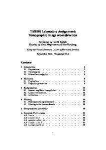
Fig. 3. The emission phantom has three regions of relative intensity (1:4:8), cold disk (left), background ellipse, and hot disk (right).
For any reconstruction, the user must set the parameters L and αa , a = 1, . . . , L. The number of classes L is assumed known for our medical examples.3 As explained earlier, αa is left as a free parameter that controls image quality by controlling a bias-variance tradeoff. For the simulations that follow, we use an empirical scheme to choose αa in which the αa are chosen to minimize the rmse (root-mean-squared error) between the reconstruction and true object. This yields a reasonable bias-variance tradeoff. Also, we note that the reconstructions are not especially sensitive to αa . A. Emission Tomography In emission tomography [11] [12], including PET (positron emission tomography) and SPECT (single-photon emission computed tomography), the goal is to reconstruct the emission object f from the projection data g. Here both the vectors g and f are lexicographically ordered with elements {gm ; m = 1, . . . , M } and {fn ; n = 1, . . . , N }, respectively. The object voxel fn , the radionuclide density, is defined as the mean number of photons emitted from voxel n into 4π s.r. per unit time. The sinogram element gm is the integer number of counts detected during the imaging time at a detector bin indexed by m. The observed sinogram g has an independent (at each detector element m) Poisson distribution with mean g¯m =
P
n
Hmn fn [13]. The system matrix H comprises elements
{Hmn ; m = 1, . . . , M ; , n = 1, . . . , N }, indicating a probability per unit time that a photon emitted from voxel n gets detected in detector bin m. A more complete model of the 3
This is an excellent assumption for medical transmission tomography but not quite as good an assumption for
medical emission tomography.
SUBMITTED TO IEEE TIP (REVISED)
15
(a)
(b)
(c)
(d)
(e)
(f)
Fig. 4. This illustrates the results of (a) FBP emission reconstruction, (b) EM emission reconstruction, (c) joint MAP emission reconstruction, and the estimated zan maps (0 ≤ zan ≤ 1) for three classes (d) a=1 (hot disk) (e) a=2 (background) (f) a=3 (cold disk).
Poisson mean would include an affine term (¯ gm =
P
n
Hmn fn + rm ) to model the effects
of randoms and scatter in PET and SPECT, but the exclusion of rm in our simulations is minor and does not substantially affect our simulations. ¯ and the independent With f now assuming the role of θ, we may use the definition of g Poisson nature of g to write the likelihood as: ΦL (g|f ) = −
X m
{gm log(¯ gm ) − g¯m }
(37)
where terms independent of fn have been dropped. The joint-MAP updates (35) and (36) may now be written using (37), and the reconstruction is carried out according to the prescription in Fig. 2. We now demonstrate the application of the joint-MAP reconstruction approach with gamma mixture priors to the emission reconstruction problem. (We retain a uniform hyperprior in these simulations.) For the emission object f , we used the 128×128 emission object shown in Fig. 3, which has three regions of relative intensities (1:4:8). (Here, darker regions are more intense.) The regions comprise a hot disk, cold disk and background ellipse. Projections were simulated at 129 angles spaced over 360 degrees with 192 detector bins per angle, and the simulated imaging accumulates 500K total counts into the sinogram.
SUBMITTED TO IEEE TIP (REVISED)
16
obj fbp em
1.5
1
0.5
0 0
20
40
60
80
100
120 obj mix
1.5
1
0.5
0 0
20
40
60
80
100
120
Fig. 5. This illustrates the profile plot of the phantom (solid line), FBP (dotted line), EM (dashed line), and joint-MAP (plus-sign) reconstructions, along central row of each image. The joint-MAP (+ sign) is displayed separately for clarity.
With the projection data g available, we can apply the joint-MAP method of Fig. 2 to reconstruct the object. For the reconstruction step of the alternating algorithm (35), we carry out the optimization by an iterative PCG (preconditioned conjugate gradient) algorithm [14], with a diagonal preconditioner. For this trial, the values of α a are chosen to be 20, 40 and 80 for the three classes, respectively. The number of classes L is assumed known and fixed at L=3 (hot disk, cold disk and background ellipse). We need an initial object estimate for the right side of the alternating algorithm (36), and here a 5-iteration ML-EM reconstruction [15] is used for the initial estimate. The initial values for {π a } and
SUBMITTED TO IEEE TIP (REVISED)
17
{βa } are less critical, and can be obtained easily from the initial estimate. 5
Ramp phantom Γ mixture
4.5
4
3.5
3
2.5 0
10
20
30
40
50
60
0.55
0.9
0.5
0.85
0.45
0.8
0.4
0.75
0.35
0.7
0.3
0.65
0.25
0.6
0.2
0.55
0.15
0.5
0.1
0.45
70
(a)
(b)
(c)
Fig. 6. (a) Profile plots along central column of ramp emission phantom (dotted line) and its joint-MAP reconstruction (solid line). Axes are intensity vs. pixel number. (b) {zan } for class a = 1. Intensity encodes values of z. (c) {zan } for class a = 2. Intensity encodes values of z. Note the gradual
transition of the z’s.
An anecdotal result of the joint-MAP reconstruction is shown in Fig. 4(c), and its final zan -maps from the mixture decomposition are displayed in Figs. 4(d)(e)(f) for three classes. These analog zan -maps constitute a segmentation of the object. For comparison, an FBP (filtered backprojection) reconstruction [16] and a ML-EM reconstruction [15] are also presented in Figs. 4(a)(b), respectively. To further illustrate reconstructions, profile plots along the central row of the reconstructions are illustrated in Fig. 5 along with a profile of the true phantom. The joint-MAP reconstruction is superior in this anecdotal simulation. It may appear that the mixture-of-gammas prior works well only with piecewise constant objects, but the result in Fig. 6 illustrates how the 2-component mixture decomposition leads to gradual spatial transitions in the zan . The phantom is a ramp intensity object ranging from a low value of 2.5 at the bottom row to 5.0 at the top row. Noisy projection data of this phantom are computed and reconstructed using our joint-MAP scheme with L = 2 and αa chosen as per our rmse scheme. Profile plots of the phantom and its reconstruction along the center column are shown in Fig. 6 (a). Figures 6(b) and (c) are images of z1n and z2n . The intensity encodes the value of z. The gradual spatial transitions in zan show that at a given location, the z’s can take on values far from 1.0 or 0.0, thus illustrating a noncommittal membership.
SUBMITTED TO IEEE TIP (REVISED)
18
B. Transmission Tomography In transmission tomography, one tries to reconstruct an image of attenuation coefficients from data obtained by projecting rays from many source locations and angles through the attenuating object. X-ray computed tomography (CT) is a familiar application, but in CT as clinically practiced, the data quality is high and analytical algorithms related to FBP can be used. Other applications, such as transmission scanning for attenuation correction in PET and SPECT [17], result in far noisier data, and estimation-theoretic approaches such as ours become useful. The transmission object is denoted by vector µ with N lexicographically ordered elements µn for each pixel n ∈ {1, . . . , N }. Note that the object θ now becomes µ. The value µn is thus the attenuation coefficient of the material in voxel n. The transmission projection data is denoted again by vector g of M lexicographically ordered elements g m , where m ∈ {1, . . . , M } indexes the detector bins as well as the ray along which the beam is attenuated. The integer value gm is the number of photons received at bin m. The problem is then to reconstruct µ from the data g. The transmission projection data g again follow an independent Poisson distribution at each bin m, but mean g¯m is now given by g¯m = um e−
P
l µ m mn n
,
(38)
where lmn is the path length of ray m as it traverses voxel n. The quantity {um ; m = 1, . . . , M }, the “blank scan”, is the number of counts received when no object is present, and can be obtained by calibration experiments. As with the emission case, terms r¯m may be added to the right side of (38) to model physical effects that arise in specific applications of attenuation correction in PET and SPECT, but their exclusion does not alter our results substantially. The likelihood for transmission tomography thus becomes ΦL (g|µ) = −
X m
{gm log(¯ gm ) − g¯m }
(39)
where constant terms have been dropped, and g¯m is given by (38). To simulate PET imaging, we used the attenuation object as shown in Fig. 7(a), which has only two values of narrow-beam attenuation coefficients appropriate at energy 511KeV,
SUBMITTED TO IEEE TIP (REVISED)
Fig. 7.
19
(a)
(b)
(c)
(d)
(e)
(f)
This shows (a) the transmission object, and the results of (b) FBP transmission reconstruc-
tion, (c) transmission reconstruction with a quadratic smoothing prior, (d) joint-MAP transmission reconstruction, and the estimated zan maps for two classes (e) a=1,(f) a=2.
0.096cm−1 for soft tissue, 0.035cm−1 for lung. The object comprises 128x128 pixels. We used transmission counts totalling 500K. Projections were simulated at 129 angles uniformly spaced over 180o , with 192 detector bins per angle. For the transmission reconstruction in the left hand side of the alternating algorithm in (35), the optimization is again carried out by an iterative PCG algorithm with a diagonal preconditioner. For the gamma mixture prior, we used L = 2 (lung, soft tissue). The initial values of πa and βa are not especially critical and were easily estimated for the transmission case from an initial object estimate. The values for αa in (lung, soft tissue) were set at (15, 60). We used a 2-iteration ML reconstruction as the initial object estimate. The reconstruction was then carried out according to the prescription in Fig. 2. Figure 7 (d) shows an anecdotal reconstruction of the joint-MAP method, while Figure 7(e)(f) are the estimated zan -maps for two classes. The zan ’s thus constitute a segmentation of the object. In addition, we ran an FBP transmission reconstruction shown in Fig. 7(b). Figure 7(c) shows a penalized likelihood reconstruction obtained with a conventional quadratic smoothing prior: Φsmooth = 12 λ P
P P n
n0 ∈N (n) (θn
− θn0 )2 . Here λ > 0
is a parameter that controls the degree of smoothing, and N (n) a neighborhood system for the voxel n. The value of the smoothing parameter was set to λ = 2000 for the best rmse result and a 4-nearest-neighbor scheme used for N (n). A profile plot of these recon-
SUBMITTED TO IEEE TIP (REVISED)
20
0.04 0.035 0.03 0.025 0.02 0.015 0.01 0.005
obj fbp mm mix
0 −0.005 0
20
40
60
80
100
120
Fig. 8. This illustrates the profile plot of the phantom (solid line - obj), FBP (dashed line - fbp), conventional smoothing prior (dotted line - mm) and joint-MAP (plus-sign - mix) transmission reconstructions, along the central row of each image. The joint-MAP reconstruction shows better performance as compared with the FBP and smoothing-prior reconstructions in terms of the qualitative profile result.
struction along central row, displayed in Fig. 8, illustrates a sense of the quality of the joint-MAP reconstruction as compared with the FBP and conventional smoothing results. VI. Discussion A. Significance of Work We have presented a joint-MAP reconstruction with a gamma mixture prior and applied it to statistical tomographic reconstructions. The gamma mixture prior assumes a clustered intensity histogram in the object, and enforces positivity naturally. Our implementation of the joint-MAP reconstruction contains an alternation between a penalized likelihood reconstruction step, and a hyperparameter estimation step (gamma mixture decomposition). In applying Hathaway’s approach [8] to the hyperparameter estimation step, one can transform the original, complex mixture objective to one that is easier to optimize. This transformation also allows the utilization of the complete data z for the reconstruction step, and leads to a simplification of the penalized likelihood optimization. Remarkably, the transformation also leads to an equivalent, independent gamma prior, where the individual mean and variance parameters of the independent gamma are
SUBMITTED TO IEEE TIP (REVISED)
21
computed from the mixture decomposition. We applied the joint-MAP reconstruction to both emission and transmission tomography, and the anecdotal results illustrate the effectiveness of the new prior. A significant aspect of our work is that it allows one to effectively use the desireable independent-but-not-identically-distributed non-mixture form of the gamma prior pdf in (9). Recall that for (10), if one were able to specify a good value for αn and βn at each pixel, then the resulting optimization (31) would be straightforward. These α n , βn determine a “external reference value”, i.e. a value at each location n, towards which the prior draws the reconstruction. However, assuming αn is set by the user to control bias variance tradeoff, there is no obvious way to choose βn . By using an independent-and-identicallydistributed mixture pdf (15), we apparently change the problem so that each voxel is drawn by the same multimodel pdf, reflecting our knowledge about the histogram of the medical object of concern. So, in our simulations, each voxel seeks a value consistent with belonging to a given class, e.g. lung or soft tissue. The resulting alternation, (17)(18), is difficult to carry out, so we transform (17)(18) to a new alternation (35)(36) that (i) preserves the fixed point of (17)(18) and (ii) introduces a new intermediate variable zan that can be interpreted as a probability of class membership of voxel n in class a. Interestingly, while (36) delivers the values for zan and βa , the update (35) is exactly of the form (31) needed for the nonmixture gamma prior (9)! In (31), the pdf is the independent, non-mixture, non-identically distributed prior pdf of (9), but now, the effective αn and βn have been determined, thus “closing the loop”. Although αa is user specified, once it has been specified, the αn are now computed automatically. Again, the iid mixture form, through transformations of the objective, results in the independent non-identically distributed non-mixture form in (31). The fixpoints remain the same, so optimizing (35)(36) is the same as the optimization (17)(18). This entire scheme does not rely on any particular property of gamma priors; we chose them for their convenient positivity-preserving properties. The entire scheme could easily be repeated with independent Gaussian pdf, for example. B. Related Previous Work In [4], an independent gamma prior was first applied in a penalized likelihood reconstruction for both emission and transmission tomography, which is equivalent to our recon-
SUBMITTED TO IEEE TIP (REVISED)
22
struction step of the joint-MAP reconstruction. However, there was no hyperparameter estimation step for computing the voxelwise hyperparameters, and these had to be specified empirically. Another pointwise Gaussian prior [18] was combined with a penalized likelihood for emission tomography. As in [4], there was no hyperparameter estimation step for computing the voxel-by-voxel hyperparameters, and the authors resorted to an empirical method of obtaining these from an initial FBP reconstruction. In [19], the gamma mixture model has been applied to estimate the proportions of classes in an SAR (synthetic aperture radar) image, where the object intensity histogram has a few (L) peaks with L known. In their work, only the hyperparameter estimation step of our alternation is performed using a slightly different derivation of the EM update equation to estimate ψ and z. In [20], an independent Gaussian mixture prior was introduced for a penalized likelihood reconstruction for emission tomography, but their approach was not a joint-MAP method with both reconstruction and hyperparameter estimation steps. The Gaussian mixture parameters were computed from a FBP reconstructed image in advance, and kept fixed throughout the reconstruction [20]. Thus there was no hyperparameter estimation step of the alternation as in our joint-MAP reconstruction. C. Issues for Future Work The free parameter L, the number of classes in the mixture model, can be confidently fixed in many applications such as thorax transmission tomography or the application in [19]. However, in other applications, such as emission tomography, the estimation of L becomes difficult. One solution is to utilize an information criterion [21], or other estimation-theoretic methods [22] and [23]. Since the mixture model is nonconvex, the result is sensitive to initial conditions. Here, 0 the initial conditions comprise the initial estimate θb , and the initial mixture parameters 0
b . For our applications to tomography, the solution is fairly robust to initial conditions. ψ
For example, one can use an FBP reconstruction as the initial estimate, and use this to get 0
b . In particular, for transmission tomography, an initial guess for the mixture parameter ψ
a reasonable mean value βa of the attenuation coefficient for each tissue class can be
obtained from reference data on tissue properties. Nevertheless, we have investigated the use of a deterministic annealing (DA) method [24] for this problem. DA methods are
SUBMITTED TO IEEE TIP (REVISED)
23
useful in finding approximate global minima to nonconvex objectives, and have found use in a wide variety of applications. To use the DA method for our case, one need only make a minor modification [24] to the update of (25). Results of applying DA illustrate a robust solution independent of the initial conditions [24]. It is relatively straightforward to incorporate hyperpriors mathematically. To incorporate hyperpriors, one may simply begin with the general formulation (5) that includes the ΦHP term, and apply all those steps used in deriving (26) and (27). Inclusion of a hyperprior leaves the reconstruction step completely unchanged. In [9], we derived modified versions of (26) and (27) to include a Dirichlet hyperprior [10] on π and a gamma hyperprior for β. However, further development is needed for testing the effects of theses hyperpriors. For our medical applications, hyperpriors on π and β have natural interpretation in terms of pdf’s (over an ensemble of patients) for cluster proportions and means. The gamma-mixture prior models voxel values as having a clustered histogram, but does not model spatial smoothness. In many applications, one would expect that a spatial correlation exists between neighboring voxels. Since the mixture prior does not assume any spatial interaction, it is possible to see some sparse misclassified (wrong z) voxels in the result. A possible way of including the spatial information is to introduce smoothing interactions on the complete data z. This involves adding smoothing terms in (24), and thus a modification of the update equation (25). Relevant approaches in [25] and [26] discuss the problem of incorporating neighbor correlations in the mixture decomposition. We will investigate this issue in future work. Appendix A. Derivation of Update equations (25)-(27) In the following we use the definition of pa as a gamma prior as in (10). The mixture decomposition problem is stated as a constrained minimization problem on (24): arg
min
ψ ∈Ω,z∈Λ
k
Φhath (z, θb |ψ) P
= arg
min
ψ ∈Ω,z∈Λ
XXn n
zan log zan
a
+zan log
o 1 πa pa (θbnk |αa , βa )
(40)
SUBMITTED TO IEEE TIP (REVISED)
24
which may be reexpressed as an unconstrained minimization via the introduction of Lagrange multipliers. By using Lagrange multipliers and adding two constraints into the objective function in (24), an overall objective function is obtained, D(z, ψ) =
XXn
zan log zan + zan log
a
n
n
+ζ(
a
X
πa − 1) −
X
κn (
X a
o 1 πa pa (θbnk |αa , βa )
zan − 1)
where Lagrange multipliers ζ and {κn } are used in imposing the constraints
P
a zan
(41) P
a
πa = 1 and
b = 1, respectively. The grouped coordinate descent is then: minimize D(z, ψ
b w.r.t. z given the previous estimate ψ
k,l−1
current estimate zbkl .
k,l−1
)
, then minimize D(zbkl , ψ) w.r.t. ψ given the
We now demonstrate that the update equations (25)(26)(27) can be obtained through
this minimization. Setting partial derivatives w.r.t. κn and zan to zero as per KarushKuhn-Tucker first order conditions [27], one obtains k,l−1
b ∂D(z, ψ ∂κn
)
=
X a
zan − 1 = 0
(42)
k,l−1
b ∂D(z, ψ ) = log zan + 1 ∂zan h i − log πbak,l−1 pa (θbnk |αa , βbak,l−1 ) − κn = 0
(43)
Solving for zan in (43), we obtain,
zan = eκn −1 πbak,l−1 pa (θbnk |αa , βbak,l−1 )
and using (42) X a
zan = 1 = eκn −1
X a
eκn −1 = P
{πbak,l−1 pa (θbnk |αa , βbak,l−1 )} 1
b ak,l−1 pa (θbnk |αa , βbak,l−1 )} a {π
(44)
(45)
kl Then by substituting (45) into (44), one can obtain (25) for zban . With the current estimate
kl zban , one can estimate the mixture parameters ψ by extremizing D(zbkl , ψ) with respect to
SUBMITTED TO IEEE TIP (REVISED)
25
ψ and the Lagrange parameters · o 1 ∂ X X n kl ∂D(zbkl , ψ) zban log = ∂ψ ∂ψ n a πa pa (θbnk |αa , βa )
−ζ(
X a
¸
πa − 1) = 0
(46)
where ∂D(zbkl , ψ) ∂ψ
= 0 =⇒
∂D(b zkl ,ψ ) ∂π ∂D(b zkl ,ψ ) ∂β
=0 =0
and the term in [square brackets] in (46) excludes terms independent of ψ. First extremizing w.r.t. πa and ζ, kl ∂D(zbkl , ψ) X zban = + ζ = 0, − ∂πa πa n
∂D(zbkl , ψ) X = πa − 1 = 0. ∂ζ a
(47)
(48)
From (47) and (48), one gets ζ = N , and the update equation for πa in (26). Then zeroing the derivative w.r.t. βa , one obtains o ∂ n X X kl ∂D(zbkl , ψ) = −zban log pa (θbnk |αa , βa ) ∂βa ∂βa n a
∂ n X X kl h αa θbnk −zban − + (αa − 1) log θbnk ∂βa n a βa io αa +αa log − log Γ(αa ) βa h X αa θbk αa i kl = = 0 zban − 2n + βa βa n =
(49)
which leads immediately to the update (27). B. Derivation for the Transformation (29) With the definition of the function z˜
z˜(θ, ψ) ≡ argmin Φhath (z, θ|ψ), P z∈Λ
(50)
the left side of (29) may be expressed as min Φhath (z, θ|ψ) = Φhath (˜z(θ, ψ), θ|ψ) P P Z∈Λ
(51)
SUBMITTED TO IEEE TIP (REVISED)
26
Using the result from Appendix-A in obtaining (25), we express z˜(θ, ψ) as πa pa (θn |αa , βa ) Aan z˜an (θ, ψ) = P = Bn b πb pb (θn |αb , βb )
(52)
where for convenience we have summarized the numerator and denominator by Aan ≡ πa pa (θn |αa , βa ) and Bn ≡ obtain
P
b
πb pb (θn |αb , βb ), respectively. Inserting (52) into (24), we
Φhath (˜z(θ, ψ), θ|ψ) = P
X h Aan
Bn
an
=−
X Aan an
Bn
log(Bn ) = −
X
where we have made use of the normalization established.
n
log(
Aan Aan 1 i )+ log Bn Bn Aan
log(Bn ) ≡ Φmix P (θ|ψ)
P
a
(53)
Aan = Bn . The relation (29) is thus
SUBMITTED TO IEEE TIP (REVISED)
27
References [1]
A. Mohammad-Djafari, “A Full Bayesian Approach for Inverse Problems,” in Proc. 15th Inter. Work. Maximum Entropy and Bayesian Methods, K. Hanson and R. Silver, Eds. 1995, pp. 135–144, Kluwer Academic.
[2]
D. Luenberger, Optimization by Vector Space Methods, John-Wiley and Sons, New York, NY, 1969.
[3]
N. Johnson, S. Kotz, and N. Balakrishnan, Continuous Univariate Distribution, vol. 1, John Wiley and Sons, 2nd edition, 1994.
[4]
K. Lange, M. Bahn, and R. Little, “A Theoretical Study of Some Maximum Likelihood Algorithms for
[5]
G. J. McLachlan and K. E. Basford, Mixture Models, Marcel Dekker, 1987.
[6]
A. P. Dempster, N. M. Laird, and D. B. Rubin, “Maximum Likelihood Estimation from Incomplete Data via
Emission and Transmission Tomography,” IEEE Trans. Med. Imaging, vol. 6, no. 2, pp. 106–114, June 1987.
the EM Algorithm,” J. Royal Statist. Soc. B, vol. 39, pp. 1–38, 1977. [7]
R. A. Redner and H. F. Walker, “Mixture Densities, Maximum Likelihood and the EM Algorithm,” SIAM Review, vol. 26, no. 2, pp. 195–239, April 1984.
[8]
R. J. Hathaway, “Another Interpretation of the EM Algorithm for Mixture Distributions,” Stat. Prob. Letters,
[9]
I.-T. Hsiao, Bayesian Image Reconstruction for Emission and Transmission Tomography, Ph.D. thesis, Dept
vol. 4, pp. 53–56, 1986. of Electrical Engineering, State Univ. of New York at Stony Brook, Stony Brook, New York 11784, USA, May 2000. [10] D. Titterington, A. Smith, and U. Markov, Statistical Analysis of Finite Mixture Distributions, John Wiley and Sons, 1985. [11] R. J. Jaszczak, “Tomographic Radiopharmaceutical Imaging ,” Proceedings of the IEEE, vol. 76, pp. 1079– 1094, September 1988. [12] M. Phelps, J. Mazziotta, and H. Schelbert, Eds., Positron Emission Tomography and Autoradiography: Principle and Applications for the Brain and Heart, Raven Press, New York, 1986. [13] H. H. Barrett and W. Swindell, Radiological Imaging: the Theory of Image Formation, Detection, and Processing, vol. I and II, Academic Press, Inc., 1981. [14] E. U. Mumcuoglu, R. Leahy, S. R. Cherry, and Z. Zhou, “Fast Gradient-Based Methods for Bayesian Reconstruction of Transmission and Emission PET Images,” IEEE Trans. Med. Imaging, vol. 13, no. 4, pp. 687–701, Dec. 1994. [15] K. Lange and R. Carson, “EM Reconstruction Algorithms for Emission and Transmission Tomography,” J. Comp. Assist. Tomography, vol. 8, no. 2, pp. 306–316, April 1984. [16] A. Rosenfeld and A. C. Kak, Digital Picture Processing, vol. 1, Academic Press, New York, 2nd edition, 1982. [17] D. L. Bailey, “Transmission Scanning in Emission Tomography,” Euro. J. Nuc. Med., vol. 25, no. 7, pp. 774–787, July 1998. [18] E. Levitan and G. T. Herman, “A Maximum A Posteriori Probability Expectation Maximization Algorithm for Image Reconstruction in Emission Tomography,” IEEE Trans. Med. Imaging, vol. 6, no. 3, pp. 185–192, Sept. 1987. [19] R. Samadani, “A Finite Mixture Algorithm for Finding Proportions in SAR Images,” IEEE Trans. Image Processing, vol. 4, no. 8, pp. 1182–1186, Aug. 1995. [20] Z. Liang, R. Jaszczak, and R. Coleman, “On Reconstruction and Segmentation of Piecewise Continuous
SUBMITTED TO IEEE TIP (REVISED)
28
Images,” in Info. Processing in Med. Imaging, A. Colchester and D. Hawkes, Eds. 1991, vol. 12, pp. 94–104, Springer Verlag. [21] Z. Liang, R. Jaszczak, and R. Coleman, “Parameter Estimation of Finite Mixtures Using the EM Algorithm and Information Criteria with Application to Medical Images,” IEEE Trans. Nuclear Science, vol. 39, no. 4, pp. 1126–1133, 1992. [22] P. Djuri´ c, “A Reversible Jump Algorithm for Analysis of Gamma Mixtures,” in Proc. SPIE: Bayesian Inference for Inverse Problems, A. Mohammad-Djafari, Ed., July 1998, vol. 3459, pp. 262–270. [23] S. Richardson and P. Green, “On Bayesian Analysis of Mixtures with an Unknown Number of Components,” J. Royal Statist. Soc. B, vol. 59, no. 4, pp. 731–792, 1997. [24] I.-T. Hsiao, A. Rangarajan, and G. Gindi, “Bayesian Image Reconstruction for Transmission Tomography Using Mixture Model Priors and Deterministic Annealing Algorithms,” in Proc. SPIE: Medical Imaging, M. Sonka and K. Hanson, Eds., Oct. 2001, vol. 4322. [25] D. Titterington, “Some Recent Research in the Analysis of Mixture Distributions,” Statistics, vol. 21, pp. 619–641, 1990. [26] S. Gopal, Deterministic and Statistical Solutions for Noninverse Problems in Image Processing, Ph.D. thesis, Department of Electrical and Computer Engineering, University of Houston, Aug. 1996. [27] D. Luenberger, Linear and Nonlinear Programming - 2nd ed., Addison-Wesley, Menlo Park, CA, 1984.