Joint Segment-level and Pixel-wise Losses for Deep Learning based

This article has been accepted for publication in a future issue of this journal, but has not been fully edited. Content may change prior to final publication. Citation information: DOI 10.1109/TBME.2018.2828137, IEEE Transactions on Biomedical Engineering 1

Joint Segment-level and Pixel-wise Losses for Deep Learning based Retinal Vessel Segmentation Zengqiang Yan, Xin Yang, and Kwang-Ting (Tim) Cheng, Fellow, IEEE

Abstract—Objective: Deep learning based methods for retinal vessel segmentation are usually trained based on pixel-wise losses, which treat all vessel pixels with equal importance in pixel-topixel matching between a predicted probability map and the corresponding manually annotated segmentation. However, due to the highly imbalanced pixel ratio between thick and thin vessels in fundus images, a pixel-wise loss would limit deep learning models to learn features for accurate segmentation of thin vessels, which is an important task for clinical diagnosis of eye-related diseases. Methods: In this paper, we propose a new segment-level loss which emphasizes more on the thickness consistency of thin vessels in the training process. By jointly adopting both the segment-level and the pixel-wise losses, the importance between thick and thin vessels in the loss calculation would be more balanced. As a result, more effective features can be learned for vessel segmentation without increasing the overall model complexity. Results: Experimental results on public datasets demonstrate that the model trained by the joint losses outperforms the current state-of-the-art methods in both separate-training and cross-training evaluations. Conclusion: Compared to the pixel-wise loss, utilizing the proposed jointloss framework is able to learn more distinguishable features for vessel segmentation. In addition, the segment-level loss can bring consistent performance improvement for both deep and shallow network architectures. Significance: The findings from this study of using joint losses can be applied to other deep learning models for performance improvement without significantly changing the network architectures. Index Terms—Segment-level loss, deep learning, retinal image analysis, vessel segmentation

I. I NTRODUCTION

R

ETINAL fundus images provide rich information about pathological changes, which can be used for diagnosis of eye-related diseases, such as macular degeneration, diabetic retinopathy, and glaucoma. Among various features in fundus images, retinal vessel features play a crucial role. Taking diabetic retinopathy as an example, microaneurysm, one fundamental symptom, generally exists along retinal vessels. For the extraction of retinal vessel features, generating an accurate segmentation of retinal blood vessels is essential. However, manual annotation by a human observer is time-consuming. Z. Yan and K.-T Cheng are with the Department of Computer Science and Engineering, Hong Kong University of Science and Technology, Clearwater Bay, Kowloon, Hong Kong (e-mail: [email protected], [email protected]). X. Yang is with the School of Electronic Information and Communications, Huazhong University of Science and Technology, Wuhan, China (e-mail: [email protected]). This work was supported by the National Natural Science Foundation of China grant 61502188, Wuhan Science and Technology Bureau award 2017010201010111 and Program for HUST Acadamic Frontier Youth Team. Copyright (c) 2017 IEEE. Personal use of this material is permitted. However, permission to use this material for any other purposes must be obtained from the IEEE by sending an email to [email protected].

Automated retinal vessel segmentation has been widely studied over decades; however, it remains a challenging task especially for thin vessels. Generally, current retinal vessel segmentation methods can be roughly divided into two main categories: unsupervised methods and supervised methods. Unsupervised methods, assuming that no manual annotation is used for reference, are generally following traditional computer vision approaches, such as filter-based [1], [2], [3] and model-based techniques [4], [5], [6]. Mendonca et al. [7] introduced four directional differential operators for centerline pixels classification, and used an iterative region growing method combined with a morphological filter for vessel segmentation. Martinez-Perez et al. [8] proposed to segment retinal vessels by calculating the first and second spatial derivatives of the corresponding intensity image followed by a multi-pass region growing method. Ali-Diri et al. [9] designed an active contour model using two pairs of contours to locate each vessel edge. Similarly, Zhao et al. [10] proposed to solve an infinite active contour model by using hybrid region information. Zhang et al. [11] proposed to segment blood vessels by a matched filter with the first-order derivative of a Gaussian filter. Lam et al. [12] adopted a multi-concavity model, including a differentiable concavity measure, a lineshape concavity measure, and a locally normalized measure, for vessel segmentation. Fraz et al. [13] also used the firstorder derivative of a Gaussian filter for vessel centerlines extraction but a multidirectional morphological top-hat operator for morphology calculation. Roychowdhury et al. [14] proposed an iterative vessel segmentation algorithm mainly based on an adaptive thresholding method. More recently, Azzopardi et al. [15] developed a modified B-COSFIRE filter by using the difference-of-Gaussian (DoG) filter and the mean shifting operation. Yin et al. [16] designed an orientationaware detector for vessel segmentation, where orientations of vessels were modeled by the energy distribution of Fourier transformation. Zhang et al. [17] proposed to solve the vessel segmentation problem by transforming a 2D image into the lifted domain via wavelet transformation, and used a multiscale second-order Gaussian filter for vessel enhancement. Generally, compared to supervised methods, unsupervised methods are less complex but also suffer from relatively lower accuracy. Supervised methods can be further classified into two groups: 1) shallow learning based methods and 2) deep learning based methods. Generally, shallow learning based methods utilize handcrafted features for classification/segmentation. Soares et al. [18] used the two-dimensional Gabor wavelet transformation response together with the pixel intensity as the

0018-9294 (c) 2018 IEEE. Personal use is permitted, but republication/redistribution requires IEEE permission. See http://www.ieee.org/publications_standards/publications/rights/index.html for more information.


feature vector, and a Bayesian classifier for vessel segmentation. Ricci et al. [19] combined a line detector with the support vector machine for vessel segmentation. Lupas¸cu et al. [20] adopted an AdaBoost classifier based on simple feature vectors consisting of local intensity, spatial properties and geometry. Marin et al. [21] trained a neural network on a 7-D vector feature space including gray-level and moment invariantsbased features. Fraz et al. [22] used an ensemble system of bagged and boosted decision trees, where each feature vector was compromised of gradient, morphology, line strength and Gabor filter response. Besides, the k-nearest neighbor classifier (KNN) [23] and the support vector machine (SVM) [24] have also been studied extensively for retinal vessel segmentation. In contrast to shallow learning based methods, deep learning based methods automatically learn features from a large amount of training data for classification/segmentation. Recently, along with the breakthrough brought by the convolutional neural networks (CNNs) [25], [26], [27], several CNNs-based deep learning models have been proposed for retinal vessel segmentation. Li et al. [28] formulated the vessel segmentation problem as a cross-modality data transformation problem, and used a deep neural network to model the transformation. Similarly, Fu et al. [29], [30] formulated the vessel segmentation problem as a boundary detection problem, which was solved by a fully convolutional neural network combined with a fully-connected Conditional Random Fields (CRFs). In [31], Maninis et al. proposed to use deep convolutional neural networks for segmentation of both retinal vessel and optic disc. Orlando et al. [32] proposed a discriminatively trained fully connected conditional random field model for vessel segmentation. Dasgupta [33] took a 28 × 28 patch centered at each pixel as the input and performed binary classification for each pixel in a fundus image. In [34], a deep learning model was trained on a large dataset generated through data augmentation and several architectures have been tested for vessel segmentation. All these deep learning models are trained based on pixelwise losses, which are calculated by pixel-to-pixel matching between every predicted probability map and a corresponding ground truth segmentation over the training set. Due to the highly imbalanced ratio between thick vessels and thin vessels in fundus images, a pixel-wise loss will inevitably guide deep learning models to emphasize more on minimizing the thickness inconsistency of thick vessels than that of thin vessels. For accurate segmentation of both thick vessels and thin vessels, one approach is to design deeper architectures to learn discriminative features for thin vessels, which however will result in higher model complexity. In this paper, we propose a segment-level loss for the training process, which is used to measure the thickness inconsistency of each vessel segment and assign corresponding weights to different pixels accordingly. Compared with pixel-wise losses, the segmentlevel loss would penalize more on the misalignment of thin vessels. Therefore, jointly adopting both the segment-level and the pixel-wise losses would enable the deep learning model to learn features more effectively for retinal vessel segmentation. Experimental results demonstrate that the model trained by the joint losses outperforms the current state-of-the-art methods.

Given a specific deep learning model, adopting the joint losses is able to effectively improve the performance compared with just utilizing the pixel-wise loss. Since the segment-level loss is independent of deep learning architectures, the proposed loss can be easily extended to other deep learning models without significantly increasing the model complexity. The paper is organized as follows. The performance of the pixel-wise loss for retinal vessel segmentation is analyzed in Section II. Section III presents details of the proposed segment-level loss and the joint-loss deep learning framework. In Section IV, we evaluate the effectiveness of the proposed joint-loss framework through multiple comparison experiments. Section IV provides a discussion about the segmentlevel loss and Section V concludes the paper. II. P IXEL - WISE L OSS IN R ETINAL V ESSEL S EGMENTATION Pixel-wise losses have been widely used for end-to-end image segmentation, including retinal vessel segmentation. A pixel-wise loss is constructed based on pixel-to-pixel matching, which directly compares the per-pixel differences between a generated probability map and the corresponding ground truth segmentation. The deviation between the output probability of a pixel and the true label is then applied for gradient calculation and back propagation. In pixel-wise losses, each pixel is treated with equal importance and the loss of each pixel is calculated separately.

Fig. 1: Exemplar results of deep learning based retinal vessel segmentation. From left to right: the fundus image, the manual annotation and the vessel segmentation generated by [30]. One common problem of pixel-wise loss based learning methods is the severe thickness inconsistency of thin vessels. As shown in Fig. 1, thickness difference between a segmented thin vessel and its manual annotation (denoted by red circles) is much greater than that between a segmented thick vessel and its ground truth (denoted by blue circles). In fact, such results are naturally caused by pixel-wise losses. Greater thickness inconsistency of thin vessels is due to the dominant amount of thick vessel pixels which makes the optimization of segmentation results of a pixel-wise loss based method largely influenced by thick vessels. If we define the vessels whose thickness is less than 3 pixels as the “thin vessels” and the rest as the “thick vessels”, nearly 77% of vessel pixels belong to the “thick vessels” and the “thin vessels” only account for 23%. As a result, a deep learning model tends to learn better features for accurate alignment of the “thick vessels”, and largely neglects to learn features for segmenting thin vessels. However, if we examine the total vessel lengths of the “thick vessels” and the “thin vessels”, the corresponding ratio would be 45% versus 55%, which is more balanced than that of pixelto-pixel matching (namely 77% versus 23%). Thus, to balance



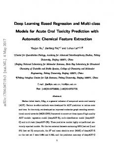
Fig. 2: The overview of the proposed joint-loss deep learning framework.

the importance between the “thick vessels” and the “thin vessels”, we propose a new segment-level loss to measure the thickness inconsistency of each vessel segment instead of the pixel-wise misalignment. Since a pixel-wise loss penalizes more on the thickness inconsistency of the “thick vessels”, the proposed segment-level loss would relatively emphasize more on the thickness consistency of the “thin vessels”. By jointly using the segment-level and the pixel-wise losses, we can balance the importance between the “thick vessels” and the “thin vessels” in the loss calculation, which enables the model to learn better features for accurate vessel segmentation. III. M ETHODOLOGY In this section, we describe in detail the design of the segment-level loss and the joint-loss deep learning framework. In the training phase, the segment-level loss and the pixel-wise loss are implemented as two branches to penalize the thickness inconsistency of both thin vessels and thick vessels. In the test phase, probability maps generated by the two branches are merged together for final segmentation. The overview of the joint-loss framework is shown in Fig. 2. A. Segment-level Loss 1) Loss Construction: We propose to measure the thickness inconsistency of each vessel segment rather than each vessel pixel. The first step is to segment the whole vessel tree into vessel segments, which is achieved based on skeletonization. Given a manual annotation I, we first apply a skeletonization method [35] to obtain the skeletons IS . Then, by detecting the intersecting pixels (namely pixels where different skeletons intersect), we canPdivide the entire skeletons IS into segments, N namely IS = i=1 Si where N is the total number of segments. It should be pointed out that, for any segment longer than a predefined maximum length maxLength, we further divide the segment into smaller segments. Exemplar results of the vessel segment generation process are shown in Fig. 3.

Fig. 3: Exemplar results of the vessel segment generation process. From left to right: the fundus image patch, the manual annotation patch, the generated skeletons and the segmented skeletons (different colors represent different segments).

For each skeleton segment Si , the corresponding vessel pixels in I that contribute to Si form a vessel segment Vi . Accordingly, the manual annotation PIN can be rewritten as a set of vessel segments, namely I = i=1 Vi . Then, the average vessel thickness TVi of each vessel segment Vi is defined as TVi =

|Vi | , |Si |

(1)

where |Vi | is the number of pixels in Vi and |Si | is the length of the corresponding skeleton segment Si . To measure the thickness inconsistency, each vessel segment Vi in I is assigned with a searching range Ri to find corresponding pixels in the predicted probability map for comparison. Given a probability map during the training process, we generate a binary map by applying a hard threshold 0.5 (namely each pixel in the probability map is classified as vessel pixel or non-vessel pixel by comparing its probability value with a hard threshold 0.5). Then, for each vessel segment Vi in I, all the vessel pixels in the binary map located within the searching range Ri form a vessel segment denoted as Vi0 . The thickness inconsistency between Vi0 and Vi is measured by defining the mismatch ratio (mr) as TV 0 − TV i 0 i , (2) mr(Vi , Vi ) = TVi



where TVi0 is the average vessel thickness of Vi0 according to the definition in (1). As TVi would be smaller for thinner vessels, the mismatch ratio is more sensitive to the thickness inconsistency of thin vessels than that of thick vessels. To construct the segment-level loss, we define a weight matrix as ( if p ∈ Vi0 , i = 1, 2, ..., N 1 + mr(Vi0 , Vi ), (3) wp = 1, otherwise, where wp is the weight of pixel p in the probability map. Then, the loss ploss of each pixel p is defined as ploss = |pprob − plabel | · wp ,

(4)

where pprob is the predicted probability value of p and plabel is the ground truth value (0 for non-vessel pixels and 1 for vessel pixels) of p in the manual annotation. According to the definition in (4), the segment-level loss is constructed based on a pixel-wise loss but with an adaptive weight matrix based on the thickness consistency measurement. 2) Hyper-parameters Selection: The proposed segmentlevel loss contains two hyper-parameters namely the maximum length of vessel segments (maxLength) and the radius of the searching range (r). The value of maxLength is determined through calculation of the thickness deviation. Given a manual annotation I, we first generate the corresponding skeleton map IS using the same skeletonization method as described in Section III.A-1). For each candidatePvalue of maxLength, we N divide IS into skeleton segments i=1 Si and I into vessel PN segments i=1 Vi according to the same method as discussed in Section III.A-1). For each skeleton segment Si and the corresponding vessel segment Vi , the thickness deviation d(Vi ) is defined as P p∈Si |tp − TVi | , (5) d(Vi ) = |Si | where p represents a skeleton pixel in Si and tp is the vessel thickness of p which is defined as the diameter of the minimum circle in I centered at p and completely covered by vessel pixels. The P overall thickness deviation d(V ) is defined as N d(V ) = N1 i=1 d(Vi ). Then, the value of maxLength is determined by selecting the value which achieves the minimum or desirable overall thickness deviation among candidate values. The radius of the searching range (r) is determined by evaluating the variations among different manual annotations [36] (as there exist location variations between vessels annotated by different observers due to the resolution limitation). Given two manual annotations I and I 0 , we first generate the corresponding skeleton maps IS and IS0 by utilizing the same skeletonization method as described in Section III.A-1). Then, given a candidate value of r, each skeleton pixel in IS is assigned with the searching range r. The value of r is determined by selecting the minimum value which achieves the maximum or desirable overlap between IS and IS0 . The potential impact of the hyper-parameters is analyzed in Section V.E.

B. Joint-loss Deep Learning Framework In terms of the deep learning architecture in the joint-loss framework, we design the basic model with reference to the U-Net [37] model, but add two separate branches to train the model with the segment-level loss and the pixel-wise loss simultaneously as shown in Fig. 2. In the training phase, kernels of the two branches are trained by the segment-level loss and the pixel-wise loss respectively, and the losses are merged together to train the shared learning architecture (UNet part) for learning better features. As discussed before, the segment-level loss penalizes more on the thickness inconsistency of thin vessels, while the pixel-wise loss mainly focuses on that of thick vessels. Therefore, simultaneously using both the segment-level loss and the pixel-wise loss is able to minimize the overall thickness inconsistency during the training process. In the test phase, since the segment-level loss and the pixel-wise loss train the model from different perspectives, we merge the corresponding probability maps predicted by the two branches by pixel-wise multiplication to generate the final vessel segmentation. As the segment-level loss is independent of deep learning architectures, the basic model in the joint-loss framework can be replaced by any other models. IV. E VALUATION A. Datasets Four public datasets DRIVE [23], STARE [38], CHASE DB1 [39] and HRF [40] are used to evaluate the proposed segment-level loss and the joint-loss framework. DRIVE consists of 40 fundus images (7 of 40 containing pathology) with a 45◦ FOV, and all fundus images in DRIVE have the same resolution of 565 × 584 pixels. The dataset is equally divided into training and test sets. As for the ground truth, two manual annotations are provided for each image in the test set, and only one manual annotation is available for each image in the training set. We follow the practice of using the annotations generated by the first observer as ground truth for performance measurement. STARE includes 20 images, 10 of which contains pathology, with the same resolution of 700×605 pixels for all images. For this dataset, as training and test sets are not explicitly specified, leave-one-out cross validation is widely used for performance evaluation. In the cross validation, each time only one fundus image is selected as the test set, and the rest 19 images are used for training. Again, manual annotations generated by the first observer are used for both training and test. Since FOV masks are not directly provided and there exists no uniform generation method, we adopt the masks provided in [21] and [32] for better comparison. CHASE DB1 comprises 28 fundus images, totally 14 pairs of images captured from different children. All images have the same resolution of 999 × 960 pixels with a 30◦ FOV. For the split of the dataset for training and test, we adopt the same strategy as described in [28] which selects the first 20 images as the training set and the rest 8 images as the test set. HRF contains 15 images of healthy patients, 15 images of patients with diabetic retinopathy and 15 images of glauco-



matous patients with a 60◦ FOV and all images have the same resolution of 3504 × 2336 pixels. In the literature, the only supervised method tested on the HRF dataset is the one reported in [32]. For a fair comparison, we constructed the same training set comprising the first 5 images of each subset and tested on all remaining images. It should be pointed out that, due to the limitation of the computational capacity, images and labels of the training set and images of the test set were downsampled by a factor of 4, and the generated results were afterward upsampled to the original size for quality evaluation. B. Preprocessing Similar to other methods, we converted each fundus image in the training set to gray scale by extracting the green channel. Then we cropped each fundus image into 128 × 128 patches with a fixed 64-pixel stride and discarded those patches in which the ratio of background pixels (pixels located outside the FOV mask) is greater than 50%. To increase the robustness and reduce overfitting, we utilized the conventional data augmentation strategies to enlarge the training set, which include flipping, rotation, resizing and adding random noise. After the data augmentation process, the numbers of training patches for the datasets DRIVE, STARE, CHASE DB1, and HRF are 7869, 8677, 4789 and 4717 respectively. C. Implementation Details The proposed joint-loss deep learning framework was implemented based on the open-source deep learning library Caffe [41]. For a fair comparison, we first trained the deep learning model without the segment-level loss branch. The initial learning rate was set at 10−4 and decreased by a factor of 10 every 30000 iterations until it reached 10−7 . Then, we trained the model with the joint losses (with two branches) under the same settings. Thus, both models were trained on the same dataset with the same total iterations. In terms of the threshold selection for quality evaluation, we adopted the same method as described in [28] where the optimal threshold was set as the threshold maximizing Acc on the training set. D. Evaluation Metrics Given a binary segmentation map under evaluation, manually annotated vessel pixels that are correctly detected as vessel pixels are denoted as true positives (TP) and those are wrongly classified as non-vessel pixels are counted as false negatives (FN). Similarly, manually annotated non-vessel pixels that are correctly classified are denoted as true negatives (TN) and those are incorrectly classified as vessel pixels are counted as false positives (FP). Then, the evaluation metrics, namely sensitivity (Se), specificity (Sp), precision (P r) and accuracy (Acc), are defined as TP TN , Sp = , TP + FN TN + FP TP + TN TP Acc = ,Pr = , N TP + FP Se =

(6)

where N = T N + T P + F N + F P . The receiving operator characteristics (ROC) curve is computed with the true positive ratio (Se) versus the false positive ratio (1−Sp) with respect to a varying threshold, and the area under the ROC curve (AU C) is calculated for quality evaluation. E. Experimental Results To evaluate the proposed joint-loss deep learning framework, we conduct experiments on the datasets DRIVE, STARE and CHASE DB1 and compare with the current state-of-theart methods. Then, we analyze the performance achieved by using the joint losses v.s. using only the pixel-wise loss. We also testify the robustness of the proposed joint-loss framework by conducting cross-training, mix-training and threshold-free segmentation experiments. Finally, we apply the joint-loss deep learning framework on the high-resolution fundus dataset HRF. Exemplar results1 are shown in the following sections. 1) Vessel Segmentation: Subjective and objective comparison results produced by different methods are shown in Fig. 4 and Table I. For the DRIVE dataset, the proposed framework achieves 0.7653, 0.9818, 0.9542 and 0.9752 for Se, Sp, Acc and AU C respectively. Compared with other state-of-the-art methods, the proposed method achieves the best results of Sp, Acc and AU C, while maintaining a top score of Se. In terms of Se, Orlando [32] achieves the best results but the score of Sp is relatively lower. Comparatively, though Se achieved by the proposed framework is 0.0244 lower, the score of Sp is 0.0234 higher. Considering the highly imbalanced ratio between vessel pixels and non-vessel pixels in fundus images, the overall accuracy of the proposed framework is much better (roughly estimated at 0.9542 v.s. 0.9457). For the STARE dataset, as no uniform FOV masks are provided, different methods might adopt different FOV masks for evaluation. In our experiment, as described in Section IV.A, we use the available FOV masks provided by Orlando [32] and Fraz [22]. Compared with the results of Orlando [32] and Fraz [22], we can effectively improve the overall performance. Compared to the best results obtained by Li [28], the results of Sp and Acc are quite similar, while the scores of Se and AU C are relatively lower. For the CHASE DB1 dataset, though no uniform FOV masks are provided, similar to other methods in practice, FOV masks can be easily generated by applying a thresholding method. According to the results in Table I, the proposed framework achieves 0.7633, 0.9809, 0.9610 and 0.9781 for Se, Sp, Acc and AU C respectively, all better than other methods. 2) Joint Losses v.s. Pixel-wise Loss: We examine the performance improvements achieved by using the joint losses versus using only the pixel-wise loss. From the experimental results in Fig. 5, we find that the probability maps generated 1 More experimental results and the trained models can be found at https://github.com/ZengqiangYan/Joint-Segment-level-and-Pixel-wise-Lossesfor-Deep-Learning-based-Retinal-Vessel-Segmentation/. To remove the possible influence of the pixel-wise multiplication in quality evaluation, we further manually run the pixel-wise multiplication on the probability map generated by the pixel-wise loss. Both objective and subjective results in subsection 2) and 4) are calculated based on the probability maps after the pixel-wise multiplication.



Fig. 4: Exemplar vessel segmentation results by the proposed joint-loss deep learning framework on the datasets DRIVE, STARE and CHASE DB1. From Row 1 to Row 4: the original fundus images, the manual annotations, the probability maps and the corresponding hard segmentation maps. TABLE I: Comparison Results on the DRIVE, STARE and CHASE DB1 Datasets Methods 2nd Human Observer Zhang [11] You [24] Fraz [13] Roychowdhury [14] Azzopardi [15] Yin [16] Zhang [17] Marin [21] Fraz [22] Li [28] Fu [29] Orlando [32] Dasgupta [33] Proposed U-Net+pixel-wise loss U-Net+joint losses

Year 2010 2011 2012 2015 2015 2015 2016 2011 2012 2016 2016 2017 2017 2017 -

Se 0.7760 0.7120 0.7410 0.7152 0.7395 0.7655 0.7246 0.7743 0.7067 0.7406 0.7569 0.7603 0.7897 0.7691 0.7653 0.7562 0.7653

DRIVE Sp Acc 0.9724 0.9472 0.9724 0.9382 0.9751 0.9434 0.9759 0.9430 0.9782 0.9494 0.9704 0.9442 0.9790 0.9403 0.9725 0.9476 0.9801 0.9452 0.9807 0.9480 0.9816 0.9527 0.9523 0.9684 0.9801 0.9533 0.9818 0.9542 0.9797 0.9513 0.9818 0.9542

AUC 0.9672 0.9614 0.9636 0.9588 0.9747 0.9738 0.9744 0.9752 0.9720 0.9752

based on the joint losses are much “cleaner” than those obtained by the pixel-wise loss. Since using joint losses is able to re-balance the importance between thick vessels and thin vessels in the training process, features learned by the joint-loss framework is more distinguishable to classify vessel pixels from non-vessel pixels. Exemplar probability maps generated by the joint losses

Se 0.8952 0.7177 0.7260 0.7311 0.7317 0.7716 0.8541 0.7791 0.6944 0.7548 0.7726 0.7412 0.7680 0.7581 0.7161 0.7581

STARE Sp Acc 0.9384 0.9349 0.9753 0.9484 0.9756 0.9497 0.9680 0.9442 0.9842 0.9560 0.9701 0.9497 0.9419 0.9325 0.9758 0.9554 0.9819 0.9526 0.9763 0.9534 0.9844 0.9628 0.9585 0.9738 0.9846 0.9612 0.9825 0.9550 0.9846 0.9612

AUC 0.9673 0.9563 0.9748 0.9769 0.9768 0.9879 0.9801 0.9696 0.9801

Se 0.8105 0.7615 0.7585 0.7626 0.7224 0.7507 0.7130 0.7277 0.7633 0.7420 0.7633

CHASE Sp 0.9711 0.9575 0.9587 0.9661 0.9711 0.9793 0.9715 0.9809 0.9807 0.9809

DB1 Acc 0.9545 0.9467 0.9387 0.9452 0.9469 0.9581 0.9489 0.9610 0.9588 0.9610

AUC 0.9623 0.9487 0.9606 0.9712 0.9716 0.9781 0.9750 0.9781

and the pixel-wise loss are shown in Fig. 6. First, the vessels segmented by the joint losses have better thickness consistency with those manually annotated vessels than those segmented by only the pixel-wise loss. The better thickness consistency is due to the fact that in the joint-loss based method the thickness consistency is measured by calculating the difference between their average vessel thickness rather than pixel-to-



Fig. 5: Results of both the cross-training and the mix-training evaluations on the datasets DRIVE (Rows 1-2), STARE (Rows 3-4) and CHASE DB1 (Rows 5-6). From left to right: the original fundus images, the manual annotations, the probability maps generated by the proposed joint-loss deep learning framework, the probability maps generated by the pixel-wise loss and the corresponding probability maps obtained by the cross-training (for the datasets DRIVE and STARE) or the mix-training (for the dataset CHASE DB1) experiments.

pixel difference. By observing the manual annotations at the pixel-wise level, we notice that precisely localizing thin vessel pixels is quite challenging even for human observers due to

the ambiguity around thin vessels as well as low contrast. Therefore, using a 2-pixel searching range to localize vessel pixels in the segment-level loss is more reasonable than



Fig. 6: Enlarged patches in the probability maps generated by the joint losses and the pixel-wise loss. From left to right: the retinal fundus patches, the manual annotation patches and the probability patches generated by the joint losses and the pixel-wise loss separately. enforcing strict pixel-to-pixel matching in the pixel-wise loss. Consequently, the segment-level loss is able to learn better features to distinguish vessel pixels from non-vessel pixels. Quantitative results with respect to different losses are shown at the bottom of Table I. For all datasets, jointly using both the segment-level and the pixel-wise losses (denoted as joint losses) can achieve better results. The improvements in Sp and Acc also demonstrate that the joint-loss framework has better ability to distinguish vessel pixels. 3) Cross-training and Mix-training Evaluations: Similar to the cross-training evaluation in [28], we testify the extendibility of the joint-loss framework by applying the model trained on one dataset to other datasets for vessel segmentation. Different from the cross-training method in [28] which retrained the deep learning model on two of the three datasets and tested on the other dataset, we directly apply the model trained on one dataset to other datasets without retraining which is more challenging and meaningful. TABLE II: Results of the cross-training evaluation Dataset DRIVE (trained on STARE)

STARE (trained on DRIVE)

Methods Soares Ricci Marin Fraz Li Proposed Soares Ricci Marin Fraz Li Proposed

Se 0.7242 0.7273 0.7292 0.7010 0.7027 0.7211

Sp 0.9792 0.9810 0.9815 0.9770 0.9828 0.9840

Acc 0.9397 0.9266 0.9448 0.9456 0.9486 0.9494 0.9327 0.9464 0.9528 0.9495 0.9545 0.9569

AUC 0.9697 0.9677 0.9599 0.9660 0.9671 0.9708

Partial results of the cross-training evaluation are shown in Fig. 5. For the DRIVE dataset, vessels in the probability maps generated by the cross-training process have better thickness consistency than those vessels in the original probability maps generated based on the pixel-wise loss only. However, since the manual annotations in the STARE dataset mainly contain thick vessels, when applying the model trained on the STARE dataset to the DRIVE dataset, the ability to detect thin vessels would be relatively limited. Comparatively, as the manual

annotations in the DRIVE dataset contain more thin vessels, when applying the model trained by the DRIVE dataset onto the STARE dataset, more thin vessels could be detected compared with the original probability maps. Comparison results of different methods on the crosstraining evaluation are provided in Table II. For the DRIVE dataset, the proposed deep learning framework outperforms other methods for Se, Sp and Acc, while the results for AU C is slightly lower. For the STARE dataset, the model trained on the DRIVE dataset achieves the best results for Se, Sp, Acc and AU C, due to that the manual annotations in DRIVE dataset contain more thin vessels so that the segment-level loss can better guide the training process for feature extraction. TABLE III: Results of the mix-training evaluation Dataset DRIVE+STARE+CHASE DB1

Se 0.7432

Sp 0.9767

Pr 0.8036

Acc 0.9501

Different from the datasets DRIVE and STARE, fundus images in the CHASE DB1 dataset are quite different in terms of both the vessel structure and the illumination. Directly applying the model trained on the DRIVE dataset or the STARE dataset to the CHASE DB1 dataset is not suitable. In this paper, we further conduct the mix-training experiment to evaluate the robustness of the proposed joint-loss framework. In the mix-training process, the training set consists of the training sets from all these datasets (for the STARE dataset we select the first 10 images as the training set), and the test set includes the rest images. Table III shows the results in the mix-training experiment. On average, the proposed joint-loss deep learning framework can achieve 0.7432, 0.9767, 0.8036 and 0.9501 for Se, Sp, P r and Acc respectively. 4) Threshold-free Vessel Segmentation: Given a probability map, instead of using the manually selected threshold to generate the hard segmentation map, we apply the Otsu [42] algorithm to automatically convert the probability map into the hard segmentation map. As shown in Fig. 7, the hard segmentation map generated by the joint-loss framework contains more vessels with better thickness consistency.

Fig. 7: Threshold-free vessel segmentation. From left to right: the fundus image, the manual annotation, the hard segmentation maps generated by models based on the joint losses and the pixel-wise loss respectively. TABLE IV: Results of threshold-free vessel segmentation Dataset DRIVE

Loss pixel-wise loss joint losses

Se 0.8284 0.8242

Sp 0.9634 0.9720

Pr 0.7711 0.8124

Acc 0.9459 0.9529

Quantitative results of the threshold-free vessel segmentation experiment are shown in Table IV. From the experimental



results, we find that the joint-loss framework is able to effectively improve the overall performance. Furthermore, the results are better than those of several state-of-the-art methods listed in Table I, which demonstrates the robustness of the segment-level loss and the joint-loss deep learning framework. 5) Performance on High-resolution Dataset: We evaluate the performance of the proposed joint-loss framework on the high-resolution fundus (HRF) image database. As shown in Fig. 8, similar to previous experimental results, using the joint losses can effectively improve the overall thickness consistency, especially for thin vessels. We also find that using the joint losses is able to learn better discriminative features to classify vessel and non-vessel pixels, which makes the generated probability maps much “cleaner”.

V. D ISCUSSION A. Dealing with Challenging Cases

Fig. 9: Retinal vessel segmentation for challenging cases. Row 1 and Row 3: from left to right are the fundus image patches, the manual annotations, the probability maps generated by the proposed network and the hard segmentation maps binarized by the Otsu [42] algorithm. Row 2: from the left to right are the fundus image patch, the manual annotations generated by the first and the second human observers and the probability map produced by the proposed model. Fig. 8: Exemplar results on the HRF database. The first row: the fundus image and the manual annotation. The second row: the probability maps generated by the pixel-wise loss and the proposed joint losses respectively.

TABLE V: Quantitative results on the HRF database Loss/Method pixel-wise loss joint losses Orlando [32]

Se 0.8084 0.7881 0.7874

Sp 0.9417 0.9592 0.9584

Pr 0.5930 0.6647 0.6630

Acc 0.9298 0.9437 -

Quantitative results of the proposed model based on different losses and the method in [32] are summarized in Table V. In this experiment, we directly set the threshold as 0.5 for hard segmentation instead of searching for an optimal threshold. Based on the results in Table V, the model trained by the joint losses can significantly improve the overall performance compared with using the pixel-wise loss. Compared to the results of Orlando [32], the proposed joint-loss framework achieves better results in all aspects. As discussed in Section IV.A, in our experiment the factor of downsampling and upsampling operations is 4 while the corresponding factor in [32] is 2. Therefore, the joint-loss deep learning framework has the potential to further improve the performance by using a smaller sampling factor.

Retinal vessel segmentation is a mature field and numerous methodologies are available. The key remaining problems that still need to be addressed include 1) vessel segmentation in the presence of lesions; 2) segmentation of low-contrast micro vessels; 3) vessel segmentation in the presence of central vessel reflex. In Row 1 of Fig. 9, we show a fundus image patch with bright lesions. Compared to the manual annotation, the probability map is slightly influenced by the presence of the lesions, but the probability values of the lesions are quite low which can be effectively removed by the automatic thresholding method. As discussed before, the segment-level loss is more sensitive to the thickness inconsistency of thin vessels, which helps learn better discriminative features, especially for thin vessels. As a result, in Row 2 of Fig. 9, although the deep learning model is trained using the manual annotations made by the first observer, the model is able to detect more micro vessels which are not annotated by the first observer but annotated by the second observer. Accurate segmentation of the low-contrast micro vessels demonstrates the robustness of the discriminative features learned by the joint-loss framework. With the presence of central vessel reflex as shown in Row 3 of Fig. 9, the proposed framework is able to segment the complete vessels with high probability values. Based on the performance on dealing with these challenging cases, we show the effectiveness of the proposed joint-loss framework for accurate vessel segmentation.



C. Revisit Se, Sp and Acc

B. Thin Vessels v.s. Thick Vessels To evaluate the effectiveness of the proposed segment-level loss, we calculate the evaluation metrics for segmentation results of thin vessels and thick vessels separately with a different searching range for matching. Given a manual annotation, vessels with the thickness less than 3 pixels are denoted as thin vessels and the rest vessels are denoted as thick vessels. To calculate the evaluation metrics Se, Sp, P r and Acc, each thin vessel is assigned with a 5-pixel searching range and pixels in a given segmentation map located within the range are counted for pixel-to-pixel matching. Similarly, each thick vessel is assigned with a 10-pixel searching range for pixel-topixel matching. The division of the vessel tree in the manual annotation is shown in Fig. 10.

Fig. 10: Division of thin vessels and thick vessels for quality evaluation. Gray ranges represent the searching ranges.

TABLE VI: Results for thin vessels v.s. thick vessels for the DRIVE dataset Vessels Thin Thick

Loss pixel-wise loss joint losses pixel-wise loss joint losses

Se 0.7527 0.7567 0.9121 0.8990

Sp 0.8945 0.9158 0.9644 0.9752

Pr 0.7014 0.7449 0.8749 0.9079

Acc 0.8607 0.8778 0.9522 0.9578

Quantitative results of different evaluation metrics for the segmentation maps generated by the automatic thresholding method described in Section IV.E-4) are shown in Table VI. According to the definitions of Sp and P r, better thickness consistency would lead to higher Sp and P r, which means that fewer non-vessel pixels in the manual annotation are incorrectly detected as vessel pixels in the segmentation map. As the proposed segment-level loss penalizes more on the thickness inconsistency of thin vessels, the joint-loss framework achieves 0.9158 for Sp and 0.7449 for P r, with an increase of 0.0213 and 0.0435 respectively compared to those of only using the pixel-wise loss. Based on the definition of the segment-level loss in (4), it would also penalize thickness inconsistency of thick vessels, which thus help improve Sp and P r of thick vessels by 0.0108 and 0.0330 respectively compared to those of only using the pixel-wise loss. Meanwhile, the results of Se are slightly lower than those of using the pixel-wise loss, which indicates that the segment-level loss is more dominating than the pixel-wise loss in the joint-loss framework. The relative weights of the segment-level loss and the pixel-wise loss should be further explored for balancing the loss calculation in the training process and for further increasing the overall performance.

Based on the definitions in Section IV.D, the evaluation metrics Se, Sp and Acc are constructed based on pixel-topixel matching, which directly compares each pair of pixels in the hard segmentation map and the manual annotation. For the deep learning models based on the pixel-wise loss, since the vessels in the probability map usually are much thicker than those in the manual annotation, a higher threshold would be adopted in order to thin the vessels to achieve better results for Se, Sp and Acc. Comparatively, the threshold used for the proposed model is quite close to 0.5, due to the pixelwise multiplication operation in the test phase. It also explains the reason why the improvements for AU C are relatively limited. Therefore, when using the metrics Se, Sp and Acc for evaluation, the quality of the output probability map might not be comprehensively evaluated, due to the selection of different thresholds. For the proposed deep learning framework, the improvements for Se, Sp and Acc mainly are due to that the joint losses enable the model to learn better discriminative features to classify non-vessel pixels. To alleviate the limitation of the pixel-to-pixel matching in quality evaluation, we further implement the f (C, A, L) function [43] to evaluate the performance of the proposed joint-loss framework on threshold-free segmentation in Section IV.E-4). In the f (C, A, L) function, parameter C penalizes fragmented segmentations by comparing the number of connected segments in the manual annotation and in the generated segmentation map. Parameter A measures the degree of overlapping areas between the manual annotation and the generated segmentation map. Parameter L compares the lengths of vessels in the manual annotation and in the generated segmentation map. To the best of our knowledge, the f (C, A, L) function has not previously been employed for quality evaluation. According to the experimental results, using the joint losses can achieve 0.8227 in terms of the f (C, A, L) function while the corresponding score obtained by using the pixel-wise loss is 0.7974, which offers another perspective for demonstrating the effectiveness of the proposed joint-loss framework. D. Architecture Independence As discussed before, we believe that the performance gain achieved by the proposed joint-loss framework is universally applicable and is somewhat independent of the choices of deep learning architectures and classifiers. To validate this point, we conduct another experiment to replace the U-Net model in the proposed joint-loss framework by a simplified FCN model [44] as shown in Fig. 11. As the simplified FCN model is quite different from the U-Net model in terms of both architecture and depth, evaluating the performance of the proposed joint-loss framework on these two vastly different deep learning models can help shed some light on the reliance of the performance gain on the choices of deep learning models. To evaluate the performance of the simplified FCN model trained by the joint losses, we conduct an experiment on the DRIVE dataset. Experimental results are shown in Fig. 12.



overall performance regardless of the deep learning architectures and classifiers. E. Hyper-parameters Evaluation As discussed in Section III.A-2), the proposed segmentlevel loss contains two hyper-parameters namely the maximum length of vessel segments (maxLength) and the radius of the searching range (r). In this section, we evaluate the impact of these hyper-parameters on the performance of the proposed joint-loss framework. TABLE VIII: Experimental results for different values of maxLength on the DRIVE dataset maxLength 8 16

Fig. 11: The overview of the simplified FCN model [44].

Fig. 12: Exemplar results generated by the FCN model [44] based on different losses. From left to right: the fundus images, the manual annotations, the probability maps generated by models based on the joint losses and the pixel-wise loss respectively. We find that the probability maps generated by using the joint losses have better vessel thickness consistency compared with those probability maps generated by the pixel-wise loss. In addition, the simplified FCN model trained by the joint losses can better identify non-vessel pixels from vessel pixels. The corresponding quantitative results of the threshold-free vessel segmentation experiment are provided in Table VII, the trend of which is quite similar to that in Section IV.E-4). Although there is a drop in Se, the joint losses can significantly improve the overall performance of Sp, P r and Acc.

Dataset DRIVE

Loss pixel-wise loss joint losses

Se 0.8338 0.8143

Sp 0.9523 0.9690

Pr 0.7224 0.7946

Acc 0.9370 0.9490

Results of the two drastically different architectures and classifiers on the threshold-free vessel segmentation experiments demonstrate that, compared to the pixel-wise loss, the proposed joint-loss framework can effectively improve the

Sp 0.9818 0.9818

Pr 0.8595 0.8587

Acc 0.9542 0.9536

AUC 0.9752 0.9756

According to the selection strategy for determining the value of maxLength in Section III.A-2), increasing the value of maxLength may increase the thickness deviation, which in turn could reduce the performance improvement achieved by the segment-level loss. As shown in Table VIII, increasing the value of maxLength from 8 to 16 slightly decreases the overall performance. On the other hand, using a smaller maxLength would increase the computational complexity. As discussed in Section III.A-2), the skeleton segmentation is accomplished by detecting intersecting pixels. Actually, observing the initial skeleton segmentation results (without using maxLength for refinement), we find that the overall thickness deviation is already quite limited. Therefore, the value of maxLength would not significantly influence the overall segmentation accuracy. To analyze the potential impact of the radius r on performance improvement, we conduct additional experiments on the DRIVE dataset by adjusting the value of r. Quantitative results in Table IX indicate that a larger r can slightly improve the overall performance as more non-vessel pixels would be penalized by both the segment-level loss and the pixel-wise loss. In the meantime, a larger r could also incur a greater computational complexity. As the improvement is limited, it is more desirable to select a small value of r which can maximize the overlap between different manual annotations and is computationally efficient. TABLE IX: Experimental results for different values of r on the DRIVE dataset Dataset DRIVE

TABLE VII: Quantitative results of the FCN model based joint-loss framework on threshold-free vessel segmentation

Se 0.7653 0.7600

r 2 5

Se 0.7653 0.7668

Sp 0.9818 0.9818

Pr 0.8595 0.8599

Acc 0.9542 0.9544

AUC 0.9752 0.9767

VI. C ONCLUSION In this paper, we analyze the limitation of pixel-wise losses for deep learning based retinal vessel segmentation. Instead of exploring deeper architectures for performance improvement, we propose a new segment-level loss jointly used with the pixel-wise loss to balance the importance between thick vessels and thin vessels in the training process. To merge the two



losses, a new deep learning framework with two branches is designed. Great performance improvements could be achieved by the joint-loss deep learning framework compared with that using only the pixel-wise loss. Experimental results on public datasets with comprehensive comparison demonstrate the effectiveness of the proposed joint-loss deep learning framework. We further conduct cross-training, mix-training and threshold-free vessel segmentation experiments to evaluate the robustness of the proposed joint-loss deep learning framework. In addition, by implementing the joint-loss framework on two different deep learning architectures, we demonstrate that the proposed loss is architecture independent and thus can be easily applied to other models for performance improvement with minor changes to the architectures. ACKNOWLEDGMENT We gratefully acknowledge the support of NVIDIA Corporation with the donation of the Titan Xp GPU used for this research. R EFERENCES [1] G. B. Kande et al., “Unsupervised fuzzy based vessel segmentation in pathological digital fundus images,” J. Med. Syst., vol. 34, no. 5, pp. 849-858, 2010. [2] T. Chakraborti et al., “A self-adaptive matched filter for retinal blood vessel detection,” Mach. Vision Appl., vol. 26, no. 1, pp. 55-68, 2014. [3] X. Yang et al., “Accurate vessel segmentation with progressive contrast enhancement and canny refinement,” in Proc. ACCV, 2014, pp. 1-16. [4] W. Li et al., “Analysis of retinal vasculature using a multiresolution hermite model,” IEEE Trans. Med. Imag, vol. 26, no. 2, pp. 137-152, Feb. 2007. [5] B. S. Y. Lam and Y. Hong, “A novel vessel segmentation algorithm for pathological retina images based on the divergence of vector fields,” IEEE Trans. Med. Imag, vol. 27, no. 2, pp. 237-246, Feb. 2008. [6] H. Narasimha-Iyer et al., “Automatic identification of retinal arteries and veins from dual-wavelength images using structural and functional features,” IEEE Trans. Biomed. Eng., vol. 54, no. 8, pp. 1427-1435, Aug. 2007. [7] A. Mendonc¸a and A. Campilho, “Segmentation of retinal blood vessels by combining the detection of centerlines and morphological reconstruction,” IEEE Trans. Med. Imag., vol. 25, no. 9, pp. 1200-1213, Sep. 2006. [8] M. Martinez-Perez et al., “Segmentation of blood vessels from red-free and fluorescein retinal images,” Med. Image Anal., vol. 11, no. 1, pp. 47-61, 2007. [9] B. Al-Diri et al., “An active contour model for segmenting and measuring retinal vessels,” IEEE Trans. Med. Imag., vol. 28, no. 9, pp. 1488-1497, Sep. 2009. [10] Y. Zhao et al., “Automated vessel segmentation using infinite perimeter active contour model with hybrid region information with application to retinal images,” IEEE Trans. Med. Imag., vol. 34, no. 9, pp. 1797-1807, Mar. 2015. [11] B. Zhang et al., “Retinal vessel extraction by matched filter with firstorder derivative of Gaussian,” Comput. Biol. Med., vol. 40, no. 4, pp. 438-445, 2010 [12] B. S. Y. Lam et al., “General retinal vessel segmentation using regularization-based multiconcavity modeling,” IEEE Trans. Med. Imag., vol. 29, no. 7, pp. 1369-1381, Jul. 2010. [13] M. M. Fraz et al., “An approach to localize the retinal blood vessels using bit planes and centerline detection,” Comput. Methods Programs Biomed., vol. 108, no. 2, pp. 600-616, 2012. [14] S. Roychowdhury et al., “Iterative vessel segmentation of fundus images,” IEEE Trans. Biomed. Eng., vol. 62, no. 7, pp. 1738-1749, Jul. 2015. [15] G. Azzopardi et al., “Trainable COSFIRE filters for vessel delineation with application to retinal images,” Med. Image Anal., vol. 19, no. 1, pp. 46C57, 2015. [16] B. Yin et al., “Vessel extraction from non-fluorescein fundus images using orientation-aware detector,” Med. Image Anal., vol. 26, no. 1, pp. 232-242, 2015.

[17] J. Zhang et al., “Robust retinal vessel segmentation via locally adaptive derivative frames in orientation scores,” IEEE Trans. Med. Imag., vol. 35, no. 12, pp. 2631-2644, Aug. 2016. [18] J. V. B. Soares et al., “Retinal vessel segmentation using the 2-D Gabor wavelet and supervised classification,” IEEE Trans. Med. Imag., vol. 25, no. 9, pp. 1214-1222, Sep. 2006. [19] E. Ricci and R. Perfetti, “Retinal blood vessel segmentation using line operators and support vector classification,” IEEE Trans. Med. Imag., vol. 26, no. 10, pp. 1357-1365, Oct. 2007. [20] C. A. Lupas¸cu et al., “FABC: Retinal vessel segmentation using AdaBoost,” IEEE Trans. Inf. Technol. Biomed., vol. 14, no. 5, pp. 1267-1274, Sep. 2010. [21] D. Marin et al., “A new supervised method for blood vessel segmentation in retinal images by using gray-level and moment invariants-based features,” IEEE Trans. Med. Imag., vol. 30, no. 1, pp. 146-158, Jan. 2011. [22] M. M. Fraz et al., “An ensemble classification-based approach applied to retinal blood vessel segmentation,” IEEE Trans. Biomed. Eng., vol. 59, no. 9, pp. 2538-2548, Sep. 2012. [23] J. Staal et al., “Ridge-based vessel segmentation in color images of the retina,” IEEE Trans. Med. Imag., vol. 23, no. 4, pp. 501-509, Apr. 2004. [24] X. You et al., “Segmentation of retinal blood vessels using the radial projection and semi-supervised approach,” Pattern Recog., vol. 44, no. 10, pp. 2314-2324, 2011. [25] A. Krizhevsky et al., “ImageNet Classification with Deep Convolutional Neural Networks,” in Proc. NIPS, 2012, pp. 1097-1105. [26] J. Long et al., “Fully convolutional networks for semantic segmentation,” in Proc. CVPR, 2015, pp. 3431-3440. [27] L. -C. Chen et al., “Semantic image segmentation with deep convolutional nets and fully connected crfs,” in Proc. ICLR, 2015. [28] Q. Li et al., “A cross-modality learning approach for vessel segmentation in retinal images,” IEEE Trans. Med. Imag., vol. 35, no. 1, pp. 109-118, Jan. 2016. [29] H. Fu et al., “Retinal vessel segmentation via deep learning network and fully-connected conditional random fields,” in Proc. ISBI, 2016, pp. 698-701. [30] H. Fu et al., “DeepVessel: Retinal vessel segmentation via deep learning and conditional random field,” in Proc. MICCAI, 2016, pp. 132-139. [31] K. K. Maninis et al., “Deep retinal image understanding,” in Proc. MICCAI, 2016, pp. 140-148. [32] J. Orlando et al., “A discriminatively trained fully connected conditional random field model for blood vessel segmentation in fundus images,” IEEE Trans. Biomed. Eng., vol. 64, no. 1, pp. 16-27, Jan. 2017. [33] A. Dasgupta, and S. Singh, “A fully convolutional neural network based structured prediction approach towards the retinal vessel segmentation,” in Proc. ISBI, 2017, pp. 18-21. [34] P. Liskowski, and K. Krawiec, “Segmenting retinal blood vessels with deep neural networks,”, IEEE Trans. Med. Imag., vol. 35, no. 11, pp. 2369-2380, Mar. 2016. [35] L. Lam et al., “Thinning methodologies-A comprehensive survey,” IEEE Trans. Patt. Anal. Machine Intell., vol. 14, no. 9, pp. 869-885, Sep. 1992. [36] Z. Yan et al., “A skeletal similarity metric for quality evaluation of retinal vessel segmentation,” IEEE Trans. Med. Imag., vol. 37, no. 4, pp. 1045-1057, Apr. 2018. [37] O. Ronneberger et al., “U-Net: convolutional networks for biomedical image segmentation,” in Proc. MICCAI, pp. 234-241, 2015. [38] A. D. Hoover et al., “Locating blood vessels in retinal images by piecewise threshold probing of a matched filter response,” IEEE Trans. Med. Imag., vol. 19, no. 3, pp. 203-210, Mar. 2000. [39] C. G. Owen et al., “Measuring retinal vessel tortuosity in 10-year-old children: Validation of the computer-assisted image analysis of the retina (CAIAR) program,” Invest. Ophthalmol. Vis. Sci., vol. 50, no. 5, pp. 20042010, 2009. [40] A. Budai et al., “Robust vessel segmentation in fundus images,” Int. J. Biomed. Imag., vol. 2013, 2013. [41] Y. Jia et al., “Caffe: Convolutional architecture for fast feature embedding,” arXiv preprint arXiv:1408.5093, 2014. [42] N. Otsu, “A threshold selection method from gray-Level histograms,” IEEE Trans. Syst. Man Cybern., vol. 9, no. 1, pp. 62-66, 1979. [43] M. E. Gegundez-Arias et al., “A function for quality evaluation of retinal vessel segmentations,” IEEE Trans. Med. Imag., vol. 31, no. 2, pp. 231239, Feb. 2012. [44] J. Long et al., “Fully convolutional networks for semantic segmentation,” in Proc. CVPR, pp. 3431-3440, 2015.


Joint Segment-level and Pixel-wise Losses for Deep Learning based

Joint Segment-level and Pixel-wise Losses for Deep Learning based

Suggest Documents

Joint Multimodal Learning with Deep Generative Models

Deep Transfer Learning with Joint Adaptation Networks

Deep Learning-Based Dynamic Watermarking for Secure

Deep Reinforcement Learning-based Scheduling for Roadside

Deep learning based computer-aided diagnosis for

Deep-Learning-Based Approach for Prediction of

Deep-Learning-Based Approach for Prediction of

Deep learning for healthcare applications based on

Multimodal deep learning approach for joint EEG-EMG data ... - arXiv

Learning-Based Joint Super-Resolution and

Transferable Joint Attribute-Identity Deep Learning for Unsupervised ...

Deep Multi-Task Multi-Channel Learning for Joint

Deep Multi-Task Multi-Channel Learning for Joint ... - Stanford University

Deep-Learning Based, Automated Segmentation

Deep Learning-Based Channel Estimation

Deep transfer learning-based hologram

Deep Learning Based Speech Beamforming

Ensemble of Feature-based and Deep learning

Joint syntactic and semantic analysis with a multitask Deep Learning ...

Joint Visual Denoising and Classification using Deep Learning

Deep Learning Based Regression and Multi-class Models for ... - arXiv

Hydraulic modeling and deep learning based flow forecasting for

A Deep Learning and Knowledge Transfer Based Architecture for ...

Deep Learning and Recurrent Connectionist-based Approaches for