advantage is particularly significant in wireless networks consisting of single-antenna nodes where spatial filtering is otherwise impossible and concurrent ...
Joint Source Power Scheduling and Distributed Relay Beamforming in Multiuser Cooperative Wireless Networks Xin Li, Member, IEEE, Yimin Zhang, Senior Member, IEEE, and Moeness G. Amin, Fellow, IEEE Center for Advanced Communications, Villanova University, USA
Abstract— This paper considers the maximization of the sum capacity of a multiuser cooperative wireless network through the joint optimization of power allocation among source nodes and distributed beamforming weights across the relay nodes. The distributed beamforming techniques offer the capability of enhancing the sum network capacity by achieving spatial multiplexing to support concurrent communications of multiple source-destination pairs. In this paper, we consider a two-hop cooperative wireless network consisting of single-antenna nodes in which multiple concurrent links are relayed by a number of cooperative nodes. When a large number of relay nodes are available, the channels of the different source-destination pairs can be orthogonalized, yielding enhanced sum network capacity. Such an advantage is particularly significant in high signal-to-noise ratio (SNR) regime, in which the capacity follows a logarithm law with the SNR, whereas exploiting spatial multiplexing of multiple links yields capacity increment linear to the number of users. However, the capacity performance is compromised when the input SNR is low and/or when the number of relay nodes is limited. Joint optimization of source power allocation and distributed relay beamforming is important when the input SNR and/or the number of relay nodes are moderate or wireless channels experience different channel variances. In these cases, the joint optimization of source power and distributed beamforming weights achieves significant capacity increment over both source selection and equal source power spatial multiplexing schemes.
I. I NTRODUCTION Cooperative communications offer spatial processing capability in wireless networks beyond the limitation of physical number of antenna sensors to yield enhanced spectral and energy efficiency [1], [2]. Among various approaches proposed in literature, distributed beamforming techniques provide spatial diversity and array gains to yield improved link liability and enhanced channel capacity [7]–[10]. It was shown in [3] and [4] that, when the number of relay nodes is very large, the channels of the different users can be asymptotically orthogonalized (referred to as distributed orthogonalization). As such, concurrent communications between multiple sourcedestination pairs can be performed with negligible multiuser interference. As a result, in a cooperative wireless network with L pairs of source/destination nodes which are relayed by K relay nodes, the sum network capacity scales as C = (L/2) log(K) + O(1), that is, the sum capacity increases linearly with the number of source-destination pairs. Such advantage is particularly significant in wireless networks consisting of single-antenna nodes where spatial filtering is
otherwise impossible and concurrent transmission within the same channel is infeasible. Achieving the full advantages of distributed beamforming, needless to say, relies on the proper selection of the relay weights. In [5], the relay weights are optimized to minimize the overall mean square error (MSE) of all users. This scheme, while is convenient to provide controlled data error rates for each user, does not necessarily maximize the data transmission efficiency of the network, particularly when some users experience channel impairment. Reference [10] optimizes the relay weights to maximize the sum capacity of all the users. It is seen that, in the presence of a large number of relay nodes, concurrent data transmission through spatial multiplexing yields higher capacity. Such advantage is particularly significant in high signal-to-noise ratio (SNR) regime, where the capacity follows a logarithm law with the SNR, whereas exploiting spatial multiplexing of multiple links yields capacity increment linear to the number of users. The optimization in [10], however, is limited to the relay nodes, whereas the uniform power allocation of all source nodes is assumed. As can be observed in [10], the scheme yields capacity degradation compared to the opportunistic source selection counterpart when the input SNR is low. The objective of this paper is, through joint optimization of power allocation among source nodes and distributed beamforming weights across the relay nodes, to maximize the sum capacity of the wireless network. Optimized source power allocation is important when the input SNR as well as the number of relay nodes are moderate, especially when the channel variances are different, for example, due to the presence of a temporary deep fade or shadowing in some wireless channels. In these cases, the joint optimization of source power and distributed beamforming weights yields significant capacity increment over both spatial multiplexing schemes with opportunistic source selection and equal source power allocation. It is pointed out in this paper, in the low SNR regime, the optimized distributed beamforming degenerates to the opportunistic source selection scheme, where a single source-destination link with the highest capacity is selected. In this paper, all the nodes considered in the multiuser cooperative wireless networks, including source, relay, and destination nodes, are assumed to use a single antenna. It is assumed that the optimization procedure is taken place
978-1-4244-4148-8/09/$25.00 ©2009 This full text paper was peer reviewed at the direction of IEEE Communications Society subject matter experts for publication in the IEEE "GLOBECOM" 2009 proceedings.
in a central station, which is usually resource-rich and is feasible to obtain the channel state information (CSI) of the network. The source power scheduling and relay weights are respectively fed to the source and relay nodes. We consider a two-hop amplify-and-forward (AF) protocol. Both relay and source nodes are assumed to have a total power constraint. In addition to spatial multiplexing, the capacity performance of time-division multiple access (TDMA) and opportunistic source selection schemes is also compared. We also examine the throughput when channels between source and relay nodes experience different variances. Fig. 1.
Notations In this paper, lowercase (uppercase) bold characters are used to denote vectors (matrices). In particular, I denotes an identity matrix with an appropriate dimension. (·)∗ denotes complex conjugate, (·)T denotes transpose of a matrix or vector, and (·)H is the conjugate transpose (Hermitian) operator. � · � denotes the the Euclidian (Frobenius) norm of a vector or a matrix. Moreover, E[·] denotes statistical mean operator. In addition, Diag[a] denotes a diagonal matrix with the elements of a as its diagonal elements, whereas diag[A] denotes a vector consisting of the diagonal elements of square matrix A. � denotes Hadamard (element-wise) product of matrices or vectors. II. S YSTEM M ODEL Refer to Fig. 1, we consider a wireless network consisting of K + 2L single-antenna nodes with L designated source-destination terminal pairs, denoted as Sl and Dl (l = 1, · · · , L), respectively, and K single-antenna relay nodes, denoted as Rk (k = 1, · · · , K). Similar to [3] and [10], we assume that 1) Source node Sl intends to communicate solely with destination node Dl ; 2) No cooperation between any of the nodes is allowed; 3) No direct link between source and destination nodes exists; 4) The nodes work in half-duplex mode, i.e., they cannot transmit and receive simultaneously; 5) Communication takes place in two hops over two separate time slots; 6) All channels are independent, frequency-flat Rayleigh block-fading with independent realizations across blocks; and 7) Transmission/reception between the nodes is perfectly synchronized. We use a two-step AF protocol, described as following. 1) During the first step (broadcast phase), the L source nodes transmit source information, sequentially (TDMA) or simultaneously (spatial multiplexing), to the (S) K relay nodes. The lth source node uses power Pl , and the channel between the lth source node to the kth relay node is denoted as hk,l (t), where l = 1, · · · , L and k = 1, · · · , K. The information symbol xl (t) is selected randomly from a code book and satisfies E(|xl (t)|2 ) = 1, E(x2l (t)) = 0, and E(x∗l (t)xn (t)) = 0 for l �= n. 2) During the second step (relay phase), the K relays amplify the respective received signals and relay them to the destination receivers. The noisy signal received at kth relay node is scaled to unit amplitude and then amplified to use relay power Pk and properly adjust the phase. We assume that the total power of the relay nodes
The diagram of the two-hop relay system.
�K is subject to constraint k=1 Pk = Pr , where Pr is the total relay power. The channel between the kth relay node and the lth receiver is denoted as gl,k (t). For notational simplicity, we will removed the timedependence expression for the channels because they are considered quasi-static and the optimization is performed over each fading block where the channel states remain unchanged. III. DATA T RANSMISSION S CHEMES In this section, we describe the data transmission schemes in a general manner that the L source nodes simultaneously transmit signals. The TDMA and opportunistic source selection schemes are then described as the special cases where only one source is active, i.e., all the other nodes are assigned a zero transmission power.
A. General Expression When the L source nodes simultaneously transmit signals, (S) with the lth source nodes uses a transmit power of Pl �L (S) P = P . The signal received at the K relay nodes s l=1 l can be written as r(t) = H[P(S) ]1/2 x(t) + v(t),
(1)
where H = [h1 , · · · , hL ] ∈ CK×L represents the channel coefficients between the L source nodes and the K relay nodes with hl = [h1,l , · · · , hK,l ]T ∈ CK×1 , (S) (S) P(S) = Diag[P1 , · · · , PL ] ∈ RL×L is a diagonal matrix which denotes the source power allocation strategy, x(t) = [x1 (t), · · · , xL (t)]T ∈ CL×1 is the source signal vector, and v(t) ∈ CK×1 is the relay noise vector observed at the K relay nodes and is assumed to be an independent and identically distributed (i.i.d.) complex Gaussian random variable vector with zero mean and unit variance. The scale factor vector, β = [β1 , · · · , βK ]T ∈ RK×1 , is obtained as ��− 12 � � = diag[HP(S) HH + I]−1/2 . β = diag E r(t)rH (t) (2) Denote w∗ = [w1 , · · · , wK ]H ∈ CK×1 as the unit-norm relay weight vector. The signal received at the the lth destination
978-1-4244-4148-8/09/$25.00 ©2009 This full text paper was peer reviewed at the direction of IEEE Communications Society subject matter experts for publication in the IEEE "GLOBECOM" 2009 proceedings.
node is expressed as � yl (t) = �Pr wH [gl �β �r(t)] + nl (t) (S) = Pr Pl wH (gl �β �hl ) xl (t) �
� sl (t) �
� � (S) + Pr wH gl �β � H¯l [P¯l ]1/2 x¯l (t) �
� jl (t) � + Pr wH [gl �β �v(t)] + nl (t), � �
B. TDMA Scheme
(3)
ul (t)
where gl = [gl,1 , · · · , gl,K ]T ∈ CK×1 is the channel vector between the relay and the lth destination node, nl (t) is the receive noise at the lth destination receiver, which is assumed to be i.i.d. complex Gaussian random variable of zero mean and unit variance. In addition,
In this scheme, a block of time is divided into L pairs of slots. In each time slot, the resource is devoted to a single source-destination link. Thus, the problem in each time slot is the same as a single-user relay network (see [7]– [9] and reference therein). Mathematically, it is equivalent to sequentially set only one non-zero diagonal element of matrix P(S) at a time. Consider the time slot t = 2L−1 in which the lth source (S) node transmits a signal stream with power Pl = Ps . The signal received at the K relay nodes is expressed as � (9) rt (t) = Ps hl xl (t) + v(t). where (·)t implies the TDMA scheme. The corresponding scaling factor vector βl becomes � �− 12 (10) βlt = diag Ps (hl hH . l + I)
Then, the signal received at the lth destination node now only contains sl (t) and ul (t), because there is no multiuser interference in the TDMA scheme. (S) (S) (S) (S) = Diag[P1 , · · · , Pl−1 , Pl+1 , · · · , PL ] ∈ C(L−1)×(L−1) , The output SNR, ρl , is expressed as
H¯l = [h1 , · · · , hl−1 , hl+1 , · · · , hL ] ∈ CK×(L−1) , (S)
P¯l
x¯l (t) = [x1 (t), · · · , xl−1 (t), xl+1 (t), · · · , xL (t)]T ∈ C(L−1)×1 . In (3), sl (t) is the desired signal, ul (t) is the overall noise (consisting of relay noise and destination receiver noise), and jl (t) denotes the multiuser interference. Thus, the output signal-to-interference-plus-noise ratio (SINR) of the lth user becomes ρl =
E{xl (t)} |sl (t)|2 E{xl¯(t)} |jl (t)|2 + E{v(t),nl (t)} |ul (t)|2
(4)
where (S)
(S)
A�l = Pl
Pr (gl glH )�(ββ T )�(hl hH l ), (5)
(S)
Bl = Pr (ββ H )�(gl glH )�(H¯l P¯l H¯H + I). l The capacity for the lth link in the underlying wireless network, conditioned with the channels H and gl is obtained as 1 (6) Cl = log2 (1 + ρl ), 2 where the factor 1/2 is used to emphasize the half-duplex signaling. Consequently, the sum capacity of the L links, conditioned to the channel states, is expressed as C=
L � l=1
Cl =
1 2
L � l=1
� log2 1 +
�
w H Al w , wH Dl w
(7)
where Dl = Bl + I. The mean value of the network capacity is obtained as C = E{hl ,gl ,l=1,···,L} C.
E{xl (t)} |sl (t)|2 (wlt )H Atl wlt , = E{v(t),nl (t)} |ul (t)|2 (wlt )H Btl wlt + 1
(11)
where Atl = Ps Pr (gl glH )�(βl βlT )�(hl hH l ), Btl = Pr (gl glH )�(βl βlH )�I.
(12)
Note that, Btl is a diagonal matrix. The optimal weight vector at the lth time slot can be obtained as [14]
w H Al w , = H w Bl w + 1
Al = Pl
ρtl =
(8)
˜l (Dtl )−1 h , (13) t −1 ˜l � �(Dl ) h √ ˜ l = Ps Pr gl � βl � hl ∈ CK×1 where Dtl = Btl + I, and h is the equivalent channel vector of user l. Substituting the above result into (11), we obtain the maximum SINR as ρtl = ˜ H (Dt )−1 h ˜l . h l l Note that, in the TDMA scheme, the capacity differs for each use. Therefore, the average capacity of the L users, conditioned with the channel states, is expressed as wlt =
Ct =
1� t 1 � t −1 ˜ ˜H hl . (14) Cl = log2 1 + h l (Dl ) L 2L L
L
l=1
l=1
The mean network capacity is obtained in a similar manner to (8). C. Opportunistic Source Selection Among the L users, the one with the optimum SNR ρtl = achieves maximum instantaneous capacity under the same transmit power and bandwidth conditions. Thus, by selecting such a best source user at each block, opportunistic information transmission can be achieved through user diversity [12], [13]. Thus, in the opportunistic source selection scheme, it remains true that the source power allocation matrix P(S) had only a single non-zero diagonal element, but the
˜ H D−1 h ˜l h l l
978-1-4244-4148-8/09/$25.00 ©2009 This full text paper was peer reviewed at the direction of IEEE Communications Society subject matter experts for publication in the IEEE "GLOBECOM" 2009 proceedings.
order is opportunistically selected, rather than sequentially determined as in the TDMA scheme. At a pair of time slots, the network capacity of the opportunistic source selection scheme is obtained as � � 1 log2 1 + ρtl , (15) C o = max Clt = max l=1,···,L l=1,···,L 2 where (·)o denotes opportunistic source selection. The mean network capacity can be formulated similar to (8).
to the non-convex and highly nonlinear nature of the problem, the optimization may not always yield global optimum. The solution depends on the initial condition used for the search. In this paper, the initial source power allocation is assumed to be uniform, and a suboptimal solution of the relay weights, developed in [10], is used to initialize the optimization process. The procedure of the joint optimization of power scheduling and relay weights is given in Table I. TABLE I J OINT O PTIMIZATION P ROCEDURE
D. Remarks We consider two special case, namely, that with a low SNR and that with a large number of relay nodes, K. When the input SNR is low, we can show that C =
L � l=1
L
2) 3)
l=1
4)
� 1 Cl = log2 (1 + ρl ) 2
1 ≈ log2 2
� 1+
L � l=1
1)
� ρl
1 ≤ log2 2
� 1+
L (S) � P l
l=1
Ps
� ρtl
5)
Define the capacity tolerance δC and the maximum (S) number of iterations Nmax . Initialize Pl := Ps /L, l = 1, · · · , L, and i := 0. Compute the suboptimal relay weights [10]. Set i := i + 1. Optimize relay weights wi∗ , subject to �wi � = 1, such that C in (7) is maximized. (S) Optimize source power allocation Pl , l = 1, · · · , L, � (S) s. t. Pl = Ps , such that C is maximized. Denote the capacity obtained in the ith iteration as C (i) . If (C (i) − C (i−1) ) < δC or i ≥ Nmax , stop; Otherwise, go to step 3.
� � 1 log2 1 + ρtl = C o . l=1,···,L 2
≤ max
(16) That is, the opportunistic source selection scheme is optimum in the sense that the network capacity is maximized. On the other hand, when K is sufficiently large, the channels corresponding to different users can be considered orthogonal. In this case, Bl in (5) reduces to Btl in (12), and Dl to Dtl as well. Thus, the conditional capacity C becomes � � L H � 1� (S) w Al w , (17) log2 1 + Pl C= 2 wH Dtl w l=1
A�l
is implicitly defined in (5). Thus, optimization of where the source power allocation subject to total source power constraint becomes a water-filling problem. Particularly, when all the users have symmetric channel conditions, equal power allocation yields the maximum network capacity. IV. J OINT O PTIMIZATION OF P OWER A LLOCATION AND R ELAY W EIGHTS Now we consider the maximization of the sum network capacity of the spatial multiplexing scheme, expressed in (7), by properly adjusting the the power allocation among the source nodes as well as the complex relay weights. Because the joint optimization of these two sets of parameters is very complicated, we consider separate optimization of them and the overall optimization is achieved iteratively. Specifically, the optimization problem is solved using the multidimensional constrained nonlinear minimization procedure solver “fmincon” provided by the standard optimization toolbox of MATLAB [15]. It is a gradient-based constrained optimizer using sequential quadratic programming, where the gradients are calculated using an adaptive finite-difference method and thus analytical gradient functions of objective and constraint functions are not compulsively required. It is noted that, due
V. S IMULATION R ESULTS Extensive simulations are carried out and comparisons are performed among the proposed joint optimization scheme (“MP-Jopt”), distributed beamforming scheme with uniform source power allocation (“MP-opt”) [10], opportunistic source selection scheme (“SS”) and TDMA (“TD”) scheme. For all the schemes, due to the use of distributed beamforming, the allocation of relay power Ps across relay nodes depends on the designed beamforming weights. Similar to [10], we define the input SNR as Ps = Pr because unit noise power is assumed. For each simulated point, 1,000 realizations of every channel are randomly and independently generated to compute the average sum capacity of the network. The channel variances are assumed to be unit, unless otherwise specified. The computation of the relay weights is based on (13) for the “TD” and “SS” schemes. For the “MP-opt” scheme, the results are obtained under optimized relay weights in the case of equal source power allocation. The joint optimized results “MPJopt” are provided using the optimization algorithm described in Table I. In Figs. 2–5, the average network capacity is plotted versus the input SNR for different schemes and varying values of L and K. It is observed that, regardless of the SNR levels, joint optimization of the source power allocation and distributed relay beamforming achieves the highest capacity among the four schemes. It is also confirmed that, in the low SNR regime, the capacity obtained from the joint optimization scheme coincides that of the opportunistic source selection scheme. Comparing Figs. 2, 3 and 4, one can see that due to the spatial diversity from the cooperation among relay nodes, all schemes benefit from the the increase of the number of relays nodes. However, as the input SNR increases, the two schemes exploiting spatial multiplexing outperform the other two schemes (SS and TD).
978-1-4244-4148-8/09/$25.00 ©2009 This full text paper was peer reviewed at the direction of IEEE Communications Society subject matter experts for publication in the IEEE "GLOBECOM" 2009 proceedings.
6
5
6 MP−Jopt MP−opt SS TD
5
3
2
1
1
5
10 SNR (dB)
15
0 0
20
Average capacity comparison (L = 2, K = 3).
Fig. 4.
5
5
15
20
MP−Jopt MP−opt SS TD
4
Capacity
Capacity
10 SNR (dB)
6 MP−Jopt MP−opt SS TD
4
3
3
2
2
1
1
0 0
5
Average capacity comparison (L = 2, K = 7).
6
Fig. 3.
3
2
0 0
Fig. 2.
4
Capacity
Capacity
4
MP−Jopt MP−opt SS TD
5
10 SNR (dB)
15
0 0
20
Average capacity comparison (L = 2, K = 4).
Fig. 5.
Figures 4 and 5 compare the average network capacity with the same number of relays nodes but different number of source nodes. While in Fig. 4 the capacity obtained from the joint optimization is very close to that obtained from the distributed beamforming scheme, implying that equal source power allocation is close to the optimum solution. In Fig. 5, however, as the number of active sources increases, the equal source power allocation scheme results in noticeable capacity reduction. Joint optimization of the source power allocation and the relay weights, therefore, becomes more important in such situations. In addition, we observe in Fig. 5 that, the most significant capacity improvement of the joint optimization scheme over the other schemes is achieved at moderate input SNR values. Figure 6 depicts the average capacity versus K for different values of L, where the input SNR is fixed to 15 dB. It is observed that, for a given value of L, the average capacity of each scheme is, asymptotically, a log-like increasing function of K. On the other hand, for a given K, the capacity of the TDMA scheme does not change with L. The capacity of the opportunistic source selection scheme slightly increases with L due to user diversity. For the “MP-opt” scheme, the capacity increases with L only when K is sufficiently large. However, for the “MP-Jopt” scheme, where joint optimization of the
5
10 SNR (dB)
15
20
Average capacity comparison (L = 3, K = 7).
source power and relay weights are performed, the capacity increases with L, regardless of the value of K. While the joint optimization scheme performs similarly to the distributed beamforming scheme for a high value of K, the former outperforms the latter when K is moderate or low. Empirically, at this SNR level, the condition is observed as K ≤ L(L + 1), in which source power allocation is important to the wireless network exploiting the distributed beamforming techniques. Furthermore, we examine the throughput performance when the channels between source and relay nodes experience different variances. Fig. 7 illustrates the throughput for various schemes, where the input SNR remains at 15 dB. The channel variance vector is respectively [1 0.5] and [1 0.5 0.3] for L = 2 and L = 3. Compared with the results depicted in Fig. 6 where a uniform channel variance is assumed, it is seen in Fig. 7 that the importance of proper source power allocation becomes more significant for the capacity enhancement when channel variances differ. This observation remains true even when K is sufficiently large. As a result, the use of joint optimization of source power allocation and distributed relay beamforming provides higher network throughput and more effective power utilization. It is worth noting that the throughput of the four schemes behaves very differently in the two examined channel
978-1-4244-4148-8/09/$25.00 ©2009 This full text paper was peer reviewed at the direction of IEEE Communications Society subject matter experts for publication in the IEEE "GLOBECOM" 2009 proceedings.
7
11 10
6
9
5 Capacity
8
Capacity
7 MP−Jopt(L=5) MP−Jopt(L=4) MP−Jopt(L=3) MP−Jopt(L=2) MP−opt(L=5) MP−opt(L=4) MP−opt(L=3) MP−opt(L=2) SS(L=5) SS(L=4) SS(L=3) SS(L=2) L=1
6 5 4 3 2 1 0 1
Fig. 6. dB).
5
10
15 20 25 Number of relays (K)
30
35
4 MP−Jopt (L=3) MP−opt(L=3) MP−Jopt(L=2) MP−opt(L=2) SS(L=2, 3) TD(L=3) TD(L=2)
3 2 1 0
40
5
10
15 20 25 Number of relays (K)
30
35
40
Fig. 7. Effect of channel variances on the average capacity (SNR=15 dB, the channel variance vector is [1 0.5] for L = 2 and [1 0.5 0.3] for L = 3).
Effect of the number of relays on the average capacity (SNR=15
R EFERENCES cases. When another worse channel with a small variance 0.3 is added into existing channels with variance vector [1 0.5], the capacity is improved when the joint optimization scheme is used, especially in the case of large K. The capacity of the “MP-opt” scheme, on the other hand, is enhanced only when K is sufficient high (e.g., K > 20 in Fig. 7), whereas the capacity of the TDMA scheme is degenerated and that of the opportunistic source selection scheme does not change. VI. C ONCLUSIONS In this paper, a joint source power scheduling and distributed relay beamforming scheme has been developed for the maximization of the sum network capacity of a multiuser cooperative wireless network. The proposed scheme outperforms all techniques compared herein, including TDMA, opportunistic source selection, and spatial multiplexing with uniform source power allocation. Compared to single-user relay schemes (TDMA and opportunistic source selection), the advantages of spatial multiplexing schemes, with optimized or uniform source power allocation, are obvious because they offer the capability of concurrently supporting multiple source streams and thus provide improved sum network capacity, particularly when the input SNR is high and/or when the number of relay nodes is high. In performing spatial multiplexing, the advantage of optimizing the source power allocation over uniform allocation is significant where both the input SNR and the number of relay nodes are not very high. Such an advantage becomes more significant when the user channels have different quality. Additionally, it is shown that, the opportunistic source selection scheme is the optimum solution in a low SNR regime.
[1] J. N. Laneman and G. W. Wornell, “Distributed space-time coded protocols for exploiting cooperative diversity in wireless networks,” IEEE Trans. Inform. Theory, vol. 49, no. 10, pp. 2415–2425, Oct. 2003. [2] A. Sendonaris, E. Erkip, and B. Aazhang, “User cooperative diversity – Part I and Part II,” IEEE Trans. Commun., vol. 51, no. 11, pp. 1927–1948, Nov. 2003. [3] H. B¨olcskei and R. U. Nabar, “Realizing MIMO gains without user cooperation in large single-antenna wireless networks,” Proc. Int. Symp. Inform. Theory, p. 18, June 2004. ¨ Oyman, and A. J. Paulraj, “Capacity scaling [4] H. B¨olcskei, R. U. Nabar, O. laws in MIMO Relay networks,” IEEE Trans. Wireless Commun., vol. 5, no. 6, pp. 1433–1444, June 2006. [5] S. Berger and A. Wittneben, “Cooperative distributed multiuser MMSE relaying in wireless ad-hoc networks,” in Proc. Asilomar Conf. Signals, Systems and Computers, Oct. 2005, pp. 1072–1076. [6] T. Abe, H. Shi, T. Asai, and H. Yoshino, “Relay techniques for MIMO wireless networks with multiple source and destination pairs,” EURASIP J. Wirelss Commun. and Networking, vol. 2006, no. 2, pp. 1–9, April 2006. [7] R. Mudumbai, G. Barriac, and U. Madhow, “On the feasibility of distributed beamforming in wireless networks,” IEEE Trans. Wireless Commun., vol. 6, no. 5, pp. 1754–1763, May 2007. [8] V. Havary-Nassab, S. Shahbazpanahi, A. Grami, and Z.-Q. Luo, “Distributed beamforming for relay networks based on second-order statistics of the channel state information,” IEEE Trans. Signal Processing, vol. 56, no. 9, pp. 4306–4316, Sept. 2008. [9] Y. Zhao, R. Adve, and T. J. Lim, “Beamforming with limited feedback in amplify-and-forward cooperative networks,” IEEE Trans. Wireless Commun., vol. 7, no. 12, pp. 5145–5149, Dec. 2008. [10] Y. Zhang, X. Li, and M. G. Amin, “Distributed beamforming in multiuser cooperative wireless networks,” ChinaCom, Xi’an, China, Aug. 2009. ¨ Oyman and A. J. Paulraj, “Power-bandwidth tradeoff in dense multi[11] O. antenna relay networks,” IEEE Trans. Wireless Commun., vol. 6, no. 6, pp. 2282–2293, June 2007. [12] P. Viswanath, D. Tse, and R. Laroia, “Opportunistic beamforming using dumb antennas,” IEEE Trans. Inform. Theory, vol. 48, no. 6, pp. 12771294, June 2002. [13] D. Tse and P. Viswanath, Fundamentals of Wireless Communications. Cambridge Univ. Press, 2005. [14] H. L. Van Trees, Optimum Array Processing, New York, NY: Wiley, 2002. [15] The Mathworks Optimization Toolbox. [Online] http://www.mathworks .com/products/optimization .
978-1-4244-4148-8/09/$25.00 ©2009 This full text paper was peer reviewed at the direction of IEEE Communications Society subject matter experts for publication in the IEEE "GLOBECOM" 2009 proceedings.