Just-In-Time Processing of Continuous Queries - CiteSeerX

Just-In-Time Processing of Continuous Queries Yin Yang

Dimitris Papadias

Department of Computer Science and Engineering Hong Kong University of Science and Technology Clear Water Bay, Hong Kong {yini, dimitris}@cse.ust.hk Abstract - In a data stream management system, a continuous query is processed by an execution plan consisting of multiple operators connected via the “consumer-producer” relationship, i.e., the output of an operator (the “producer”) feeds to another downstream operator (the “consumer”) as input. Existing techniques execute each operator separately and push all results to its consumers, without considering whether the consumers need them. Consequently, considerable CPU and memory resources are wasted on producing and storing useless intermediate results. Motivated by this, we propose just-intime (JIT) processing, a novel methodology that enables a consumer to return feedback expressing its current demand to the producer. The latter selectively generates results based on this information. We show, through extensive experiments, that JIT achieves significant savings in terms of both CPU time and memory consumption.

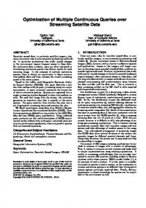
I. INTRODUCTION In typical data stream applications, including wireless sensor networks [5], road traffic monitoring [3] and publish-subscribe services [10], data continuously flow into a DSMS. Users of the DSMS pose long-running queries, whose results are incrementally evaluated as data records arrive or expire. To answer such a query, the DSMS runs an execution plan consisting of multiple basic operators (e.g., selections, joins) connected via the producer-consumer relationship, where the output of the producer comprises the input of the consumer. Besides a few top-level operators whose results are directly presented to the user, most operators generate output for the sole purpose of feeding their consumers. Figure 1.1a shows an example of a continuous query expressed in CQL [1]. Tuples from three streaming sources A, B and C are joined to detect a certain event. As a real-world example, an abnormal combination of readings from close-by humidity, light and temperature sensors may trigger the alarm in a factory [5]. The clause “RANGE 5 minutes” specifies that each record is alive for exactly 5 minutes, after which it expires and is purged from the system. Figure 1.1b illustrates a possible execution plan for this query consisting of two binary join operators Op1 and Op2 (denoted by ovals). Op1 joins sources A and B, whereas Op2 joins the result of Op1 (i.e., A B) with source C. Op1 (Op2) is the corresponding producer (consumer) of Op2 (Op1) respectively. The rectangles SA, SB (SAB and SC) denote operator states of Op1 (Op2), which hold tuples that came in the past, and

are still valid. For example, at any time instant, SB holds B tuples that have arrived in the last 5 minutes. A more detailed explanation of streaming join operators and their states is given in Section II. SELECT * FROM A [RANGE 5 minutes], B [RANGE 5 minutes], C [RANGE 5 minutes] WHERE A.x = B.x AND A.y = C.y

Op2:Consumer SAB A B C SC Op1:Producer SA A B A

SB B

Source C

(a) CQL Expression (b) Execution plan Figure 1.1 Continuous query example An important fact overlooked in most previous work is that the producer does not have to generate a result that is not used by any of its consumers. We illustrate it with the tuple arrival sequence of Table 1.1. Suppose a record a1 from source A arrives at time 1, while there are three join partners b1, b2, b3 of a1 in SB, but no matching tuples of a1 in SC. Under conventional methods, operator Op1 (i.e., the producer) uses a1 to probe (i.e., to identify join partners) SB, generating three partial results a1b1, a1b2 and a1b3. Operator Op2 (the consumer) then uses each of them to probe SC, obtaining no results since no tuple in SC matches a1. Tuple a1 and partial results a1b1, a1b2, a1b3 are inserted into operator states SA and SAB respectively. Note that, at the current time instant, it is not necessary for the producer (Op1) to generate any of the three intermediate results a1b1, a1b2, a1b3 since the consumer (Op2) is unable to obtain any output with them. Yet, CPU time and memory resources are spent on computing and storing them. If no matching tuple of a1 appears in C before the expiration of these intermediate results, the resources spent on them are wasted1. Table 1.1 Example tuple arrival sequence Timestamp Tuple (attribute values) 0 b1(x=1), b2(x=1), b3(x=1) 1 a1(x=1, y=100) 2 b4(x=1) 3 a2(x=1, y=100) 1

Partial results — a1b1, a1b2, a1b3 a 1b 4 a2b1, a2b2, a2b3, a2b4

Some query processing algorithms (e.g., M-Join [23]) do not store intermediate results. In this case the resources for producing a1b1, a1b2, a1b3 are wasted regardless of whether matching C tuples of a1 arrive in the future.

Next, suppose that at time 2 a new record b4, matching a1, arrives while there are still no join partners of a1 in SC. By probing SA with b4, Op1 generates a partial result a1b4, and subsequently performs a futile probing against SC. Similar to the previous three partial results, the computation of a1b4 is a waste of resources. Furthermore, the sheer presence of a1 enlarges the size of SA, making the probing against SA more expensive even for incoming B tuples that do not match a1. Finally, assume that at time 3, a new record a2 arrives with identical values on the join attributes x and y as a1. This time, 4 intermediate results (a2b1-a2b4 shown in Table 1.1) are generated and 4 pointless probes against SC are performed. In general, as tuples like b4 and a2 keep coming, an increasing number of unwanted intermediate results are produced each time. This problem is amplified when more sources participate in the query. Motivated by these observations, we propose Just-InTime (JIT), a novel processing approach that dynamically adjusts the execution of producer operators based on the requirements of their consumers. Applying JIT to our example, after Op2 finds out that a1b1 cannot generate join results due to the lack of matching tuples in SC, it sends a feedback to Op1, which immediately suspends the processing of a1. Meanwhile, Op1 stores a1 in a blacklist instead of SA to prevent future join partners of source B (e.g., b4), or similar tuples of A (e.g., a2), from generating unnecessary intermediate results. If a matching tuple of a1 arrives later in C, Op2 reports a change of demand to Op1, which then resumes the processing of a1 and related tuples (e.g., b4, a2), producing the required partial results in a just-in-time fashion. We show experimentally that JIT achieves significant performance gains, especially for queries with comparatively high selectivity. The rest of the paper is organized as follows. Section II surveys related work. Section III outlines the general framework of JIT. Section IV provides efficient implementation of key components of JIT. Section V discusses JIT in various query plans. Section VI contains an extensive experimental evaluation. Finally, Section VII concludes with directions for future work. II. RELATED WORK Existing work in the data stream literature can be classified into two categories: the first aims at summarizing streaming data into synopsis structures (e.g., histograms, wavelets, sketches) and using them to provide fast, approximate answers to specific aggregate queries (e.g., [15, 12]); the second focuses on the design of general-purpose DSMSs (e.g., Aurora [2, 8], STREAM [1], TelegraphCQ [4], etc.) with formal semantics, expressive query languages and efficient query processing techniques. This work falls in the latter category, as a novel approach to continuous query processing.

A fundamental difference between a traditional DBMS and a DSMS is that the latter faces infinite inputs from the streaming sources, which cannot be handled by blocking operators such as joins [19]. To tackle this problem, most DSMSs adopt the sliding-window semantics. Specifically, for each source, the user specifies a window of fixed length. In the example of Figure 1.1, all three sources are assigned a window of 5 minutes. Hereafter, for simplicity we assume the existence of a global window of length w. Each incoming tuple t is associated with a timestamp t.ts, and is considered alive during the lifespan of [t.ts, t.ts+w). Accordingly, two input tuples t and t′ with timestamps t.ts and t′.ts can join only if |t.ts–t′.ts| ≤ w. A join result t with component inputs t1, …, tm is usually assigned a timestamp of t.ts = maxmi=1ti.ts [1]. For example, in Figure 1.1b, let ab be an output tuple of the operator A B, produced by joining a (from A) and b (from B). Then, ab.ts is the later timestamp between a.ts and b.ts. Assuming that a.ts and b.ts represent the arrival time of the two tuples, then ab.ts can be interpreted as the earliest time that ab can be created. In addition, most DSMSs require the results of a query to be reported according to their temporal order: for any two result tuples t and t′, t is reported before t′ if and only if t.ts ≤ t′.ts. Query processing in a DSMS entails the construction and execution of a query plan. This work focuses on the execution part. Under this context, one of the most extensively studied problems is join processing, which is inherently more complex than single-input operators such as selections and projections. The state-of-the-art binary join algorithms (e.g., [16]) involve three steps: purgeprobe-insert. Consider for instance, the operator A B in Figure 1.1b. An incoming tuple a from input stream A first purges tuples of SB, whose timestamp is earlier than a.ts-w; then, it probes SB and joins with its tuples; finally, a is inserted into SA. An m-way join can be computed through m–1 binary join steps. For example, the query plan in Figure 1.1b answers a 3-way join with two binary join operators, Note that such a plan (commonly referred to as X-Join [11]) stores intermediate join results (e.g., those of A B) in the operator state (SAB). In contrast, an M-Join [23] plan, illustrated in Figure 2.1a, does not store any intermediate results. Instead, tuples in each source go through a linear path of m–1 operators to join with tuples from other sources. This approach costs less memory than the XJoin, but more CPU time due to repeated computations of intermediate results. Adaptive caching [11] provides a tradeoff between memory and CPU resources, resembling a tree of M-Join operators. Finally, the Eddy architecture [4], shown in Figure 2.1b, features the novel Eddy operator that dynamically routes source tuples and intermediate results to appropriate operators to complete their processing. The proposed algorithms can be applied to all these types of join plans.

C SC Op2

C SC Op4

B SB Op6

B SB Op1

A SA Op3

A SA Op5

A

B

Op1 Op2 A SA

B

SB

Op3 C

SC

Eddy

C A

B

C

(a) M-Join (b) Eddy Figure 2.1 Example of alternative m-way join plans A plethora of optimizations for continuous query processing have been proposed in the literature. When there are numerous operators in the system, operator scheduling (e.g., [9]) finds the best execution order for minimizing memory consumption and maximizing throughput. Adaptive query processing techniques (e.g., dynamic plan migration [25, 24]) dynamically adjust the query to optimize performance in the presence of changing stream characteristics. When the system has insufficient CPU or memory resources to process the query completely, load shedding (e.g., [22]) or operator spilling (e.g., [20]) aims at generating a maximal (or wellrepresented) subset of the actual results. In case of multiple running queries, performance can be improved through shared execution (e.g., [14]) and query indexing (e.g., [18, 6]). Finally, novel hardware, such as the Cell processor [13], can be used to improve performance. Our work is orthogonal to the above methods. Demand-driven operator execution (DOE) [21], recently proposed in the context of stream keyword search, suspends a join operator whenever (i) one of its states becomes empty, or (ii) all its consumers are suspended. As we demonstrate later, this is an extreme case that a producer generates only unwanted intermediate results; thus, DOE is subsumed by JIT. Furthermore, DOE focuses on keyword search systems, following some specific assumptions (e.g., the execution plan is always a left-deep tree), whereas the proposed solutions are generally applicable to all query plans. III. GENERAL FRAMEWORK OF JIT Section III-A describes JIT at an abstract level. Section III-B deals with operator scheduling issues. Section III-C discusses feedback propagation in plans where the same operator acts both as a consumer and producer. A. Main Concepts Let Q be a continuous query registered in the DSMS, and EP(Q) be the execution plan of Q constructed by the query optimizer. For ease of presentation, hereafter we focus on the case that EP(Q) is a tree of binary join operators, i.e., an X-Join plan [11], and discuss more complicated plans in Section V. JIT does not rely on any assumptions about the shape of EP(Q) (which can be leftdeep, right-deep or bushy), or the value distributions of the records arriving from the data sources. Let OC, OP ∈

EP(Q) be two operators forming a consumer-producer relationship, i.e., the output of OP is one of OC’s inputs. JIT considers the case where OC is selective with respect to the inputs supplied by OP. This means that several partial results generated by OP never contribute to the output of OC, which we call fruitless partial results (FPRs). In Figure 1.1, assuming that during a1’s lifespan, a matching tuple never appears in C, then a1b1, a1b2, etc., are all FPRs with respect to consumer Op2. However, given an intermediate result t from OP, it is impossible for OC to determine whether t is an FPR or not before its expiration, because a join partner of t may arrive at a later time. On the other hand, OC knows those partial results that are currently not needed, which we call non-demanded partial results (NPRs). In the running example, at timestamp 1, a1b1, a1b2, a1b3 are NPRs with respect to Op2. Clearly, each NPR has two possible destinies: (i) to be matched by a future partner, or (ii) to become a FPR after its expiration. JIT postpones the generation of NPRs of type (i) until they are demanded, i.e., when a matching partner arrives, and eliminates the production of type (ii) NPRs altogether. JIT exploits the observation that there is a broad class of partial results that can be detected as NPRs before their generation. Their common characteristic is that they contain minimal non-demanded sub-tuples (MNSs), such that any output of OP that is super-tuple of an MNS must be an NPR. In the running example, a1 is an MNS; joining a1 with any B tuple leads to an NPR. We require a nonempty MNS to be minimal, i.e., not to contain another MNS as sub-tuple. The empty tuple Ø is sub-tuple of any record. It is possible for Ø to be a valid MNS, when the opposite operator state (of OP) at OC is empty. In this case, all results computed by OP are NPRs, and OP can be simply suspended, achieving the same effect as DOE [21]. Figure 3.1 visualizes the relationship between FPR, NPR and MNS.

minimum sub -tuple of non -demanded evolve non -demanded into partial result sub-tuple (NPR ) (MNS) super -tuple of

Fruitless partial result (FPR) Matched partial result

Figure 3.1 Concepts of FPR, NPR and MNS According to JIT, consumer OC detects MNSs during join processing, and reports them to OP as a suspension feedback. In our example, consumer Op2 processes input a1b1, identifies a1 as an MNS, and sends a feedback f = to producer Op1. Once OP receives such a feedback, it immediately stops generating results that are super-tuples of the specified MNSs. Continuing the example, Op1 stops joining a1 with B tuples, thus avoiding intermediate results a1b2, a1b3, a1b4. Furthermore, if later a new tuple a2 arrives, with identical attribute value on y (the join attribute of A and C) as a1, it is not joined with B, eliminating the generation of more NPRs.

Similar to an NPR, an MNS may be matched by a later partner. Therefore, OC stores all detected MNSs in an MNS buffer until their expiration, and probes each incoming tuple from the opposite input against the MNS buffer. The MNS buffer may be organized as a hash table, or other index structure, to speed up the probing. Whenever OC finds a matching tuple t of an MNS s, it removes s from the MNS buffer, and sends a resumption feedback containing s to producer OP. Upon receiving this message, OP immediately starts generating the set Ss of super-tuples of s that have not been produced before, and returns Ss to OC. After obtaining Ss from OP, OC joins t with Ss to generate results, and appends Ss to the corresponding operator state. We call the producer’s reactions to both kinds of feedback collectively as dynamic production control. Using the running example, suppose that at timestamp 4, a new tuple c1 (c1.y = 100) arrives from source C. Op2 finds that c1 matches MNS a1, and sends the feedback f′ = to Op1. Op1 joins a1 and a2 (whose processing is also suspended since its y attribute is identical to a1) with tuples in SB, obtaining Sa1 = {a1b2, a1b3, a2b4, a2b1, a2b2, a2b3, a2b4}. Note that a1b1 is not included in Sa1 because it has already been generated (before a1 is found as an MNS). Op1 returns Sa1 to Op2, which joins it with c1, generating 7 results. Finally, all tuples in Sa1 are appended to SAB. The general framework of JIT is flexible, in that it can be adapted to the stream (e.g., arrival rate) and query characteristics (e.g., operator selectivity). Specifically, a consumer OC may choose not to detect all MNSs for a given input. Intuitively, detecting more MNSs gives better guidance to producer OP (at the expense of higher cost at OC), but does not affect the correctness of the output. Furthermore, OP may decide to ignore the message and keep producing NPRs. B. JIT and Operator Scheduling Just-in-time processing necessitates the cooperation of OC, OP and the DSMS’s operator scheduler to maximize its performance. In this section we present some scheduling policies starting with the case that f is a suspension feedback. At the time that OC issues f, it is possible that OP is currently working on producing NPRs specified by f. In the running example, when Op2 sends f = , Op1 may be joining a1 with another tuple in SB, say b2. Upon receiving f, JIT requires OP to suspend its current work and immediately handle f. OP resumes previous work only after finishing dealing with f. In the example, after handling f, Op1 learns that a1 is an MNS and stops joining it with SB. Moreover, it is also desirable for the scheduler to assign OP a higher priority than its upstream operators while processing f, because (as discussed in Section III-C) OP may propagate the feedback to them.

A complication arises when the DSMS places an interoperator queue between each pair of consumer / producer operators to store the partial results not yet processed by the consumer (in order to enable more flexible operator scheduling). After OC identifies an MNS s, super-tuples of s may have already been produced and stored in the queue QCP between OC and OP. Note that OC cannot simply delete them from QCP because they are considered “future inputs” at this moment. For instance, let t be a super-tuple of s. There may exist another tuple t' in the opposite queue (i.e., the queue of the other OC input) such that t' matches t and t'.ts ≤ t.ts, meaning that t and t' can generate a result. In our prototype, we process these super-tuples as normal input since the size of an inter-operator queue is usually small. When OC detects one of them, it sends a feedback to OP specifying s as an MNS. If OP has already suspended generating such NPRs, it simply ignores the message. Next we discuss resumption messages. Recall that a resumption feedback is issued by OC during the processing of an incoming tuple t, requesting OP to produce a set S of suppressed inputs. Because of the temporal ordering requirement, OC must process t before generating results for subsequent inputs. This means that if OC finishes the purge-probe-insert routine of t before S is ready, it has to wait for OP to compute S. This waiting may lead to temporary silence of OC’s output and, in a distributed setting (where OC and OP are on different sites) idle CPU cycles. JIT takes several measures to eliminate this waiting. First, for each incoming tuple t, OC first probes t against the MNS buffer before the opposite operator states. The rationale is that if matching MNSs of t are found, OC continues to purge / probe t against the opposite operator state, and at the same time OP starts to compute the demanded partial results S. OC waits for OP only if the latter does not complete computing S before the former finishes probing t against the corresponding operator state. Second, after OC sends a resumption feedback to operator OP, the scheduler assigns OP a higher priority than OC. Finally, similar to the case of suspension messages, upon receiving a resumption feedback, OP immediately suspends its current work, computes S, and then resumes the previous job. We summarize the timeline of the production resumption process in Figure 3.2. Probe t against the MNS buffer and find a matching MNS s OC

Send feedback to OP

Probe t against the opposite operator state

Get Ss from OP and join t with Ss time

OP Previous work

Get feedback Suspend Compute Send Ss Resume and previous super-tuples to OC continue from OC previous work work Ss of s

Figure 3.2 Timeline of production resumption

C. Feedback Propagation In complex query plans, the producer OP may also have upstream operators that supply its inputs. In Figure 3.3a, Op3 is simultaneously a producer for Op4, and a consumer with regard to Op1 and Op2. A subtlety in this situation is that the dynamic production control performed by an operator (as a producer) may change its demand for inputs (as a consumer). Consider the tuple arriving sequence of Figure 3.3c. The join predicate checked at Op4 is illustrated in Figure 3.3b. For simplicity, we assume that all tuples shown in the sequence (a1-e1) match each other. Initially, records b1 and c1d1 are present in operator states SB and SCD respectively. Then, tuple a1 from source A is joined with b1, generating a1b1, which is subsequently joined with c1d1, producing a1b1c1d1. SABCD

(b) Join Predicate at Op4

Op3 SAB

SCD

Op1 SA A

SB SC B

(A.x = E.x) ∧ (B.y = E.y) ∧ (C.z = E.z) ∧ (D.w = E.w)

Op4 SE

C

Op2 SD D

E

Timestamp

Tuple

0 1 2

b1, c1d1 a1 e1

(a) Query plan (c) Tuple arrival sequence Figure 3.3 A 5-way join example Now at Op4, suppose SE has matching records of b1 and d1, but not a1 and c1. Op4 thus sends a feedback to Op3. Responding to the feedback, Op3 stops joining tuples containing a1 or c1 (e.g., a1b1, c1d1 respectively) with their corresponding partners (inputs from Op2 and Op1). Consequently, Op3’s demand for inputs has changed; in particular, it does not want inputs that are super-tuples of a1 or c1 any longer. Hence, it propagates the feedback to Op1 and to Op2. Similarly, when e1 (matching a1 and c1) arrives at time 2, Op3 receives the resumption feedback from Op4. It then propagates to Op1 and to Op2, obtains the required inputs from them, and computes the partial results requested by Op4. Scheduling policies are more complex in the presence of feedback propagation, but follow the general idea described in Section III-B: (i) an operator always propagates a feedback before handling it, (ii) upon receiving a feedback, an operator suspends its current job and handles the feedback, (iii) an operator handling a suspension feedback has higher priority over its upstream ones, and (iv) an operator handling a resumption message computes the tuples requested by its consumer, while at the same time expecting inputs from its producers (to which it has propagated the feedback) and has a lower priority over these producers. Figure 3.4 summarizes the general framework of JIT, which consists of two procedures: Process_Input (performed by the consumer) and Handle_Feedback (by the producer).

Process_Input (Tuple t, Operator OP) // Consumer // INPUT = t : an input tuple // OP: the producer operator that generates t 1. Let St (So) be the operator state corresponding to t (opposite of t) 2. Let NBo be the MNS buffer opposite of t 3. Initialize MNS set Π to empty 4. Purge NB, and probe t against NB 5. For each MNS s ∈ NBo matching t 6. Remove s from NBo and add s to Π 7. If Π is not empty 8. Send a feedback to OP 9. Assign OP a higher priority than the current operator 10. Purge So and probe t against So, generating results 11. Compute the MNS set Ω = Identify_MNS(t) 12. If Ω is not empty, send a feedback to OP 13. Insert t into St 14. If Π is not empty 15. Retrieve input set SΠ corresponding to Π from OP 16. Join t with SΠ, generating results 17. Append SΠ to So Handle_Feedback (Feedback f, Operator OC) // Producer // INPUT = f: a feedback of the form // OC: the consumer that sends f 1. Suspend current operation 2. Propagate_Feedback(f) 3. If command is suspend, call Suspend_Production(Π, OC) 4. Else, call Resume_Production(Π, OC) 5. Resume the operation suspended at Line 1

Figure 3.4 General framework of JIT Lines 10 and 13 in Process_Input materialize the purgeprobe-insert processing routine for a given input t. Before that, the consumer probes t against the MNS buffer NB and sends the resumption feedback (Lines 1-9). The response of this feedback is retrieved later (Lines 14-17), according to the asynchronous messaging protocol described above. After probing the opposite state So, the consumer detects MNSs of t, and sends a suspension feedback, if any MNS is found. Regarding the producer, the only change is that it now handles the pre-emptive job of responding to feedback. Specifically, it first propagates the feedback to upstream operators (Line 2), and performs appropriate operations depending on the type of the feedback (Lines 3-4). Two important aspects of JIT are left open in the above framework: (i) on the consumer’s side, function Identify_MNS and (ii) on the producer’s side, functions Propagate_Feedback, Suspend_ Production and Resume_Production. We call them collectively as the feedback mechanism and discuss it in detail in the next section. IV. IMPLEMENTATION OF THE FEEDBACK MECHANISM Section IV-A describes MNS detection by the consumer operator. Section IV-B presents the dynamic production control, i.e., the producer’s reactions to feedback. A. MNS Detection A suspension feedback is initiated when a consumer OC identifies that some input tuple t does not have join partners, in which case OC sends a message to the corresponding producer OP of t. MNS(t) is the set of minimal non-demanded sub-tuples contained in t. Any sub-tuple of t that has the potential to belong to MNS(t) is called candidate non-demanded subtuple (CNS). A CNS can only contain components that appear in the join predicate of OC. Consider, for instance, that the consumer is the top join of Figure 1.1, i.e., OC =Op2 and t = ab (received from OP =Op1). Given the join predicate A.y = C.y at Op2, the CNSs are a and Ø2. In the more complex scenario of Figure 3.3, for an input t = abcd of Op4, there are 16 CNSs, e.g., Ø, a, ab, abc, abcd, etc., which are all combinations of components a, b, c, and d involved in the conditions of Op4: (A.x = E.x) ∧ (B.y = E.y) ∧ (C.z = E.z) ∧ (D.w = E.w). CNSs can be organized in a lattice, where each node corresponds to a CNS and nodes are connected by the "sub-tuple" relationship. Figure 4.1 illustrates the lattice for input t = abcd in the example of Figure 3.3.

ab

abc

abcd abd acd

ac

ad

a

b

level 4

bcd

level 3

bc

bd

cd

c

d

level 2

level 1

level 0 Ø Figure 4.1 Example CNS lattice

Two important properties of the lattice are (i) if a CNS/node s is determined to be an MNS, then none of its ancestors can be an MNS because they are not minimal (although they are all NPRs), and (ii) given a node s above Level 1 and a tuple t′, s matches t′ if and only if all its children match t′. Regarding property (i), if one of a, b, ab or ac is an MNS, abc cannot be an MNS since it contains an MNS as a sub-tuple. Similarly, for property (ii), if abc matches a tuple t' both ab and ac must match t'. Let So be the opposite state of t in OC. Identify_MNS uses the CNS lattice to efficiently determine (i) given a CNS s and a tuple t′∈So, whether s matches t′, and (ii) given a CNS s that has no matching tuples in So, whether s is minimal. The basic idea of the algorithm is to match all nodes with each tuple t′∈So, and subsequently report minimal CNSs that do not have a matching partner. Figure 4.2 illustrate the pseudo-code. As a special case, if So is empty, Identify_MNS reports Ø as the only MNS and returns immediately. Otherwise, it initializes each node of the CNS lattice L to alive, meaning that it has the potential to become an MNS. Then, for each tuple t' ∈ So, the algorithm tests every Level 1 node s against t'. If s matches t', s is marked as matched; otherwise, it is set to unmatched. Next, it proceeds to examining nodes in increasing order of their level. Each node is marked as matched, if all its children are matched. After completing 2

Recall from Section III-A that the empty tuple Ø is a valid MNS, when the opposite operator state of OC is empty.

the traversal of L for t', all matched nodes are set to dead, and Identify_MNS proceeds to the next tuple in So. When all tuples in So have been processed, the algorithm picks nodes that are both alive and minimal. Specifically, it starts from Level 1 and reports all alive nodes as MNSs. Then, it checks higher nodes level by level. For each alive node s, if any of its children is an MNS or non-minimal, s is marked as non-minimal; otherwise, s is reported as an MNS. Identify_MNS (Record t) // Consumer // INPUT = t : an input record from producer; 1. Let St (So) be the operator state corresponding to t (opposite of t) 2. If So is empty, report Ø as the only MNS and return 3. Let L be the CNS lattice of t 4. Initialize all nodes in L to be alive 5. For each record t′ ∈ So 6. For each Level 1 node s ∈ L, mark s as matched if it matches t′, and unmatched otherwise 7. For l = 2 to top level of L 8. For each s on level l of L 9. Mark s as matched if all its children are matched, and unmatched otherwise 10. Set a node to dead if marked as matched during Lines 6-9 11. Report each Level 1 node that is alive as MNS 12. For l = 2 to top level of L 13. For each s on level l of L 14. Mark s as non-minimal if any of its children is MNS or non-minimal; otherwise, report s as MNS

Figure 4.2 Algorithm Identify_MNS Note that a matched node may become unmatched during the processing of a subsequent tuple. On the other hand, once a node dies, it stays so for the entire execution. Consider again input t = abcd of Op4 in Figure 3.3 and a tuple e1 in SE = So such that a.x = e1.x. The processing of e1 will set node a to matched (Line 6) and then dead (Line 10). Now assume a subsequent tuple e2 in SE such that c.z = e2.z. During the processing of e2, node c becomes matched and dies. However, node ac remains unmatched (and alive) because the status of a has switched to unmatched (but still dead) for e2. Identify_MNS can be combined with a nested loop join of t and So, since both probe t against all So records. Furthermore, when the join condition at OC contains equijoin predicates, its performance can be accelerated using Bloom filters [7] on So. Specifically, a Bloom filter comprises of (i) BF[1..k], a k-bit string of binary values, and (ii) a set of l hash functions h1, h2, …, hl, each of which maps all values in the domain to integers in [1, k]. Given a set of values V, BF[i] is 1 if there exists v ∈ V and 1≤j≤l such that hj(v) = i, and 0 otherwise. Clearly BF[i] can be built with a single scan of V. Given a value v, if there exists 1≤j≤l such that BF[hj(v)] is 0, one can be sure that v does not exist in the value set V. Continuing the example, a Bloom filter maintained on E.y (E.z, E.w) is capable of detecting (some) b (c, d) sub-tuples that do not match any tuple in SE, respectively, and thus are MNSs. This method has lower computation cost than Identify_MNS, but may not detect all MNSs.

B. Dynamic Production Control In this section we focus on the handling of feedback messages by Suspend_Production, Resume_Production and Propagate_Feedback. In all these procedures, each MNS in the feedback is handled independently. Thus, without loss of generality, we assume that the feedback contains only one MNS. Let operators OL and OR supply the left and right inputs of OP, respectively. Depending on the schema of results produced by OL and OR, an MNS is classified into two types: a Type I MNS is a sub-tuple of results generated exclusively by OL or OR, whereas a Type II MNS is a sub-tuple of the combination of results produced by OL and OR. In the example of Figure 3.3, OP = Op3, OL = Op1 and OR = Op2. Sub-tuples a, ab and c belong to Type I, while ac belongs to Type II. We also distinguish two cases for suspension of production. The first refers to conventional suspension feedback, i.e., an operator completely stops producing NPRs containing an MNS. On the other hand, a markresult feedback requires the producer to mark, rather than to suspend production of, super-tuples of the specified NPRs. A mark-result message is generated for type II MNSs. Consider, for instance, that Op3 in Figure 3.3 wants to stop MNS {ac}, generated from inputs OL = Op1 (for a) and OR = Op2 (for c). Op3 passes to Op1 and to Op2. Op1 (Op2) then marks every output that is a super-tuple of a (c), respectively. At Op3, marked AB tuples from Op1 containing a as a sub-tuple are not joined with marked CD tuples from Op2 containing c, thus eliminating a*c* output (although permitting results such as a*c1* and a1*c*). Let s be an MNS of Type I from OL. Suspend_Production scans the operator state SL of OL, extracting all super-tuples of s, and moves them to a blacklist BL associated with SL. If right before handling the feedback, OP was joining a super-tuple t of s, t is also inserted to BL. After finishing feedback handling, OP continues to process the next input tuple t′ succeeding t. In the example of Figure 1.1 and Table 1.1, if Op1 receives while joining a1 with b2 ∈ SB, it moves a1 to blacklist BA, and then continues with the next incoming tuple b4. The blacklist BL is organized as follows. Each entry of BL consists of an MNS s and a list of s’s super-tuples, each associated with a timestamp specifying when they are inserted to BL. For a suspension feedback, incoming tuples from OR are not joined with BL, so as to prevent the generation of NPRs. For a mark-result feedback, however, new tuples from OR have to join BL, generating marked outputs. Hence, when there is hash table or index structure maintained on SL, it is desirable to extend the structure to cover the "marked" tuples in BL for efficient probing. Recall from the example of Figure 1.1 that OP can detect new MNSs (e.g., a2) if they have the same join attribute values as an existing MNS s. This is realized by

two additional operations. First, during the scan of the operator state (SL) to identify super-tuples of s, OP also finds those records in SL that contain a sub-tuple s′ with identical join attributes as s, and moves these records to BL as well, under the entry for s. Second, when a new record t (e.g., a2) arrives from OL, OP compares it with MNSs in BL. If t contains such a sub-tuple s′, t is inserted to BL. For a suspension feedback, no further processing of t is necessary, whereas for a mark-results feedback, t is joined with SR, marking the results. For a Type II MNS s, Suspend_Production first decomposes it into sL and sR. Then, OP (i) scans both states SL and SR, moving super-tuples of sL and sR to black lists BL and BR, respectively, and (ii) sends mark-results messages to OL and OR. If the process is initiated by a suspension feedback, each marked incoming tuple only probes against SL (or SR), while an unmarked tuple joins both SL/SR and BL/BR. Otherwise, (the process is initiated by mark-result), a marked input is also probed against SL/SR, and the outputs are marked. Next, we discuss Resume_Production, assuming that s is a Type I sub-tuple of OL’s results. First, OP finds the entry with MNS s in BL. For an unmark-results feedback, OP simply moves all super-tuples of s to SL. For a resumption feedback, OP joins each super-tuple t of s with tuples in SR whose arrival timestamps are larger than the suspension time of t, and inserts t to SL. In the example of Figure 1.1, suppose BA contains a1 and a2, when Op1 receives from Op2. Op1 moves both tuples back to SA, and joins a1 with b2-b4 and a2 with b1-b4. Note that a1 is not joined with b1 because the suspension time of the former (1) is not earlier than the arrival time of the latter (1), suggesting that when a1 is inserted into BA, it has already been joined with b1. Type II MNSs are handled in a similar manner. During feedback propagation, OP simply relays a Type I MNS to OL and/or OR in its original form, e.g., if it receives , Op3 passes to Op1. For an MNS s of Type II, OP first decomposes s into two sub-tuples sL and sR based on the schema of OL and OR’s results, e.g., sub-tuple ac is decomposed into a and c. Then, it sends sL to OL and sR to OR, using a mark-result feedback. Similarly for a resumption feedback containing a Type II MNS s, OP passes sL and sR to OL and OR respectively, enclosed in unmark-result feedback, which stops the marking process. We end this section with a note that practical implementations of the above functions have a high degree of flexibility since JIT serves as an optimization, not a core requirement, for query processing. For example, an implementation may choose not to handle Type II MNSs, or not to detect new MNSs based on known ones. V. EXTENSIONS TO OTHER OPERATORS AND PLANS So far we have focused on binary tree plans and the case that both the consumer and producer operators are joins. However, the applicability of JIT is not restricted to this

context. We first extend JIT to operators beyond joins. When OP is not a join operator, it may be unable to perform dynamic production control; on the other hand, if an upstream operator O′ of OP is a join, OP can simply pass feedback from a downstream consumer OC to O′, and the latter then adjusts its production accordingly. A consumer OC can be an arbitrary operator as long as it is able to detect MNSs using an algorithm similar to Identify_MNS (see Section IV-A). For instance, consider the plan of Figure 5.1a, in which OC = Op2 is a selection. For the sequence of inputs in Table 1.1, Op2 = σA.x>200 detects a1 as an MNS once it receives a1b1 from Op1. It thus sends to Op1, which stops joining a1 with records in SB. Instead of maintaining a black list, Op1 can simply delete a1, as Op2 will never issue a resumption message. In Figure 5.1b, consumer Op2 joins its inputs from Op1 with a static relation RC, rather than another streaming source. JIT applies to this plan in a similar way to the case of Figure 5.1a, i.e., Op2 may send suspension, but not resumption, feedback. Op2 σA.x>200 Op1 SA A B

SB

Op2 A B C RC Op1 SA A B SB

A B B (a) OC is a selection (b) OC is a static join Figure 5.1 Alternative plans

A

Next we discuss JIT in plans with complex operators, specifically, M-Join and Eddy. As shown in Figure 2.1a, an M-Join involves multiple “half join” operators, each of which has only a single operator state (e.g., operator B has only one state SB). Such operators are similar to the join in Figure 5.1b, except that the operator states (e.g., SB) get updated as tuples arrive and expire in the corresponding stream (e.g., B). Therefore, resumption feedback is necessary as new matching partners of an MNS may appear later. The processing of this feedback, however, is simpler than the case of binary stream joins, in that the consumer does not request inputs from the producer from such messages. For example, in the leftmost operator path in Figure 2.1a, suppose Op2 has issued a suspension feedback to its Op1 specifying a1 as an MNS. Later a matching partner c1 of a1 arrives and is inserted to SC. Because c1 is processed along a different path (Op5 and Op6), Op2 is not activated and thus does not need super-tuples of a1 from Op2. The Eddy architecture (Figure 2.1b) is similar to MJoins in the sense that tuples are processed in the “half join” units (called STeMs in [4]), but now there are no fixed consumer-producer connections between them. We view every STeM as both a consumer and a producer. Once an MNS s is detected, it is sent back to the Eddy that propagates it to STeMs, whose operator state may contain s as a sub-tuple. For instance, MNS a1 is propagated to STeM Op1, which then puts a1 in a

blacklist. Resumption feedback can be handled in a similar manner. Finally, the JIT logic can also be programmed into user defined aggregates (UDAs), which let the user organize simple operations with control flows, achieving Turing-complete expressive power [19]. VI. EXPERIMENTAL EVALUATION We have implemented JIT in C++ following the PIPES [17] stream management framework, and performed all experiments on a Pentium 4 3.0G CPU with 2GB of RAM. For each set of experiments, we generate synthetic data for N streaming sources, and process a continuous join query over the N sources with a clique-join predicate. Specifically, there is an equi-join condition between each pair of sources; every tuple from any of the N sources contains N–1 columns corresponding to the other N–1 sources. For example, if there are 4 sources A, B, C and D, the join predicate is (A.x1=B.x1) ∧ (A.x2=C.x2) ∧ (A.x3=D.x3) ∧ (B.x4=C.x4) ∧ (B.x5=D. x5) ∧ (C.x6 = D.x6), where x1-x6 are distinct columns. Unless otherwise specified, each source has an average tuple arrival rate of λ tuples per second, and each column value is a random integer uniformly distributed in the range [1..dmax]. Intuitively, a larger dmax leads to a more selective join because the probability of two values to be equal is smaller. A sliding window of size w is applied to all sources. We investigate the effect of JIT on two different categories of binary join trees: bushy and left-deep, both of which are commonly used in practice. Table 6.1 summarizes all query plans used in the experiments. A plan is executed twice, each time for 5 hours application time, with and without JIT. We refer to the execution without JIT as REF (for reference solution). The two solutions are compared in terms of total CPU time and peak memory consumption. All joins are implemented using the nested loop algorithm [16]. Table 6.2 summarizes the ranges of all parameters, with default values in bold. Table 6.1 Execution plans N Bushy Plan Left-Deep Plan 3 (A B) C  4 (A B) (C D) ((A B) C) D 5 ((A B) (C D)) E (((A B) C) D) E 6 ((A B) (C D)) (E F) ((((A B) C) D) E) F 7 ((A B) (C D)) ((E F) G)  8 ((A B) (C D)) ((E F) (G H)) 

Table 6.2 Parameters under investigation Range & Default Bushy Left Deep window size w (min) 10, 15, 20, 25, 30 5, 7.5, 10, 12.5, 15 0.4, 0.7, 1, 1.3, 1.6 0.4, 0.7, 1, 1.3, 1.6 stream rate λ (/sec) #sources N 4, 5, 6, 7, 8 3, 4, 5, 6 max data value dmax 100, 150, 200, 250, 300 30, 40, 50, 60, 70 Parameter

We first present the results for the bushy plans. Figure 6.1 shows the CPU time and memory consumption as a

function of the window size w. In terms of CPU time, JIT outperforms REF by more than an order of magnitude (Figure 6.1a), while saving up to 62% of memory (Figure 6.1b). Note that the performance gains are amplified with increasing w. The advantage of JIT mainly comes from the reduction of FPRs (i.e., unnecessary partial results). In general, a longer window has two effects on the number of FPRs: (i) it leads to a larger number of total intermediate results, causing more FPRs; (ii) it increases the chance that an intermediate result has matching partners, reducing FPRs. The former effect prevails because it is magnified through multiple join operators, while the latter is always linear to w. 10000CPU time (secs)

12000 Memory (KBs)

REF

REF

4000

JIT

2000

10

15

w (mins) 25 30

20

w (mins)

0 10

15

20

25

30

(a) CPU time (b) Memory consumption Figure 6.1 Overhead vs. window size w (bushy plan) Figure 6.2 plots CPU and memory cost against the stream rate λ. The effect of λ is similar to that of the window size w, and as λ increases, JIT yields larger savings compared to REF. Intuitively, a rapid stream rate leads to more intermediate results, many of which are not demanded by their corresponding consumers and are, therefore, eliminated by JIT. 10000CPU time (secs)

12000 Memory (KBs)

REF

10000

1000

8000

JIT

100

0.4

0.7

1

1.3

0.7

1

1.3

λ 1.6

(a) CPU time (b) Memory consumption Figure 6.2 Overhead vs. stream rate λ (bushy plan)

8000 Memory (KBs) 7000

REF

6000

1000

REF

5000

100

10 4

4000

JIT

5

6

7

150

3000 N 2000 8 4

JIT N 5

6

200

250

300

3000 2000

JIT 100

150

dmax

200

250

300

Having established the superiority of JIT in high selectivity settings and bushy plans, we next investigate its performance for low selectivity and left-deep plans. As shown in Table 6.2, the default dmax used in this set of experiments is as low as 50, compared with 200 in the previous settings. In order not to overload the system, we apply smaller w (window size) and N (number of sources), and feed stream D (C when N = 3) with values from [1..102dmax]. Figures 6.5 and 6.6 illustrate the results for varying w and λ, respectively. Due to the relatively low selectivity, many intermediate results have matching partners and, thus, the effect of JIT is less pronounced. Nevertheless, JIT still has a clear advantage over REF, especially for higher values of w and λ.

7

600 400 200 0

Figure 6.3 studies the effect of the number N of streaming sources. Again, JIT outperforms REF by large margins on both metrics and its overhead increases slower with N. An interesting observation is that in terms of memory consumption, REF exhibits a step-wise pattern, i.e., the plans with 4 and 5 (also 6 and 7) inputs consume similar amounts of memory, which reflects the nature of the bushy plans. In JIT, however, this pattern does not exist because many intermediate results are eliminated. 10000CPU time (secs)

100

800 0.4

4000

dmax

1000

JIT

2000 0

REF

5000

JIT

100

1200

4000

λ 1.6

7000 6000

1400 CPU time (secs)

REF

6000

10

8000

CPU time (secs) 1000

(a) CPU time (b) Memory consumption Figure 6.4 Overhead vs. max data value dmax (bushy plan)

6000

10

9000 Memory (KBs)

REF

10

8000

JIT

100

1

10000

10000

1000

1

Figure 6.4 demonstrates the impact of dmax, i.e., the maximum column value for each tuple. Recall that a large dmax leads to a small output size. Consequently, fewer intermediate results are generated and the overhead of both JIT and REF decreases. Note that in JIT, when dmax exceeds 200, both the CPU cost and the memory consumption remain relatively stable because, after this point, very few intermediate results are produced.

8

(a) CPU time (b) Memory consumption Figure 6.3 Overhead vs. number of sources N (bushy plan)

5

7.5

5000 Memory (KBs) 4500 4000 3500 3000 REF 2500 2000 w (mins) 1500 JIT 1000 5 7.5 10 12.5 15

REF JIT

10

12.5

w (mins) 15

(a) CPU time (b) Memory consumption Figure 6.5 Overhead vs. window size w (left-deep plan) 1600 CPU time (secs) 1400 1200 1000 800 600 400 200 0 0.4 0.7

6000 Memory (KBs) 5000 4000

REF

JIT

2000

JIT 1

REF

3000

1.3

λ 1000 0.4 1.6

0.7

1

1.3

λ 1.6

(a) CPU time (b) Memory consumption Figure 6.6 Overhead vs. stream rate λ (left-deep) Figure 6.7 compares JIT and REF with respect to the number of streaming sources (N). JIT outperforms REF and scales more gracefully as N grows, especially in terms of CPU time. Finally, Figure 6.8 illustrates the effect of dmax. REF incurs high cost for low selectivity (dmax < 50), whereas JIT, successfully handles even very low selectivity.

600

3000

CPU time (secs)

500

REF

400

[3] Memory (KBs)

REF

2500

300

JIT

2000

[4]

200 JIT

100 0

1500

3

4

N 6

5

1000

3

4

N 6

5

(a) CPU time (b) Memory consumption Figure 6.7 Overhead vs. number of sources N (left-deep) 1200

4500

CPU time (secs)

30

[7]

3000

REF dmax JIT 40

50

REF

2500

400

0

Memory (KBs)

3500

800

200

60

70

JIT

2000

[8]

1500 1000

dmax 30

40

50

60

70

(a) CPU time (b) Memory consumption Figure 6.8 Overhead vs. max data value dmax (left-deep) VII. CONCLUSION This paper proposes JIT, a novel framework for continuous query execution. JIT eliminates unnecessary intermediate results through the collaboration between the consumer and producer operators, thus achieving significant savings in terms of both CPU time and memory consumption. We first present a general framework of JIT, including (i) a feedback mechanism, (ii) scheduling policies that maximize parallelism, and (iii) a message propagation scheme to amplify the effects of JIT. Then, we describe efficient implementations of key components of JIT, specifically, the feedback generation algorithm at the consumer and the dynamic production control routines performed by the producer. A comprehensive set of experiments confirm that JIT improves performance, often by orders of magnitude. This work opens several directions for future work. So far, we have focused on the case that the exact results are required. The first interesting problem is to integrate JIT with approximate query processing methods, such as load shedding [22]. Furthermore, we intend to investigate the application of JIT in wireless sensor networks [5], where the elimination of unnecessary partial results is critical for minimizing network transmissions and prolonging the battery life of sensors. ACKNOWLEDGEMENTS This work was supported by the grant HKUST 6184/05E from Hong Kong RGC. REFERENCES [1]

[2]

[6]

4000

1000

600

[5]

Arasu, A., Babu, S., Widom, J. The CQL Continuous Query Language: Semantic Foundations and Query Execution. VLDB J., 15(2), 2006. Abadi, D. J., Carney, D., Cetintemel, U., Cherniack, M., Convey, C., Lee, S., Stonebraker, M., Tatbul, N., Zdonik, S. B. Aurora: a New Model and Architecture for Data Stream Management. VLDB J. 12(2), 2003.

[9]

[10] [11] [12] [13] [14]

[15] [16] [17] [18] [19]

[20] [21] [22] [23]

[24] [25]

Arasu, A., Cherniack, M., Galvez, E. F., Maier, D., Maskey, A., Ryvkina, E., Stonebraker, M., Tibbetts, R. Linear Road: A Stream Data Management Benchmark. VLDB, 2004. Avnur, R., Hellerstein, J. M. Eddies: Continuously Adaptive Query Processing. SIGMOD, 2000. Abadi, D., Madden, S., Lindner, W. REED: Robust, Efficient Filtering and Event Detection in Sensor Networks. VLDB, 2005. Agarwal, P., Xie. J., Yang, J., Yu, H. Scalable Continuous Query Processing by Tracking Hotspots. VLDB, 2006. Bloom, B. Space/Time Trade-offs in Hash Coding with Allowable Errors. Communications of the ACM, 13(7):422-426, 1970. Balakrishnan, H., Balazinska, M., Carney, D., Cetintemel, U., Cherniack, C., Galvez, E., Salz, M., Stonebraker, M., Tatbul, N., Tibbets, R., Zdonik, S. Retrospective on Aurora. VLDB J., 13(4), 2004. Babcock, B., Babu, S., Datar, M., Motwani, R., Thomas, D. Operator Scheduling in Data Stream Systems. VLDB J, 13, 2004. Bizarro, P., Babu, S., DeWitt, D., Widom, J. ContentBased Routing: Different Plans for Different Data. VLDB, 2005. Babu, S., Munagala, K., Widom, J., Motwani, R. Adaptive Caching for Continuous Queries. ICDE, 2005. Cormode, G., Garofalakis, M. Sketching Probabilistic Data Streams. SIGMOD, 2007. Gedik, B., Yu, P., Bordawekar, R. Executing Stream Joins on the Cell Processor. VLDB, 2007. Krishnamurthy, S., Franklin, M. J., Hellerstein, J. M., Jacobson, G. The Case for Precision Sharing. VLDB, 2004. Korn, F., Muthukrishnan, S., Wu, Y. Modeling Skew in Data Streams. SIGMOD, 2006. Kang, J., Naughton, J. F., Viglas, S. Evaluating Window Joins over Unbounded Streams. ICDE, 2003. Krämer, J., Seeger, S. PIPES – a Public Infrastructure for Processing and Exploring Streams. SIGMOD, 2004. Lim, H., Lee, J., Lee, M. Whang, K., Song, I. Continuous Query Processing in Data Streams Using Duality of Data and Queries. SIGMOD, 2006. Law, Y.-N., Wang, H., Zaniolo, C. Query Languages and Data Models for Database Sequences and Data Streams. VLDB, 2004. Liu, B., Zhu, Y., Rundensteiner, E. Run-time Operator State Spilling for Memory Intensive Long-Running Queries. SIGMOD, 2006. Markowetz, A., Yang, Y., Papadias, D. Keyword Search on Relational Data Streams. SIGMOD, 2007. Tatbul, N., Zdonik, S. Window-aware Load Shedding for Aggregation Queries over Data Streams. VLDB, 2006. Viglas, S., Naughton, J. F., Burger, J. Maximizing the Output Rate of Multi-Way Join Queries over Streaming Information Sources. VLDB, 2003. Yang, Y., Krämer, J., Papadias, D., Seeger, B. HybMig: A Hybrid Approach to Dynamic Plan Migration for Continuous Queries. TKDE 19(3), 2007. Zhu, Y., Rundensteiner, E., Heineman, G. T. Dynamic Plan Migration for Continuous Queries Over Data Streams. SIGMOD, 2004.