Justifications for Logic Programs under Answer Set Semantics

Under consideration for publication in Theory and Practice of Logic Programming

1

Justifications for Logic Programs under Answer Set Semantics Enrico Pontelli, Tran Cao Son, and Omar Elkhatib Department of Computer Science New Mexico State University epontell|tson|[email protected]

submitted 24 May 2007; revised 22 March 2008, 19 September 2008; accepted 27 November 2008

Abstract The paper introduces the notion of off-line justification for Answer Set Programming (ASP). Justifications provide a graph-based explanation of the truth value of an atom w.r.t. a given answer set. The paper extends also this notion to provide justification of atoms during the computation of an answer set (on-line justification), and presents an integration of on-line justifications within the computation model of Smodels. Off-line and on-line justifications provide useful tools to enhance understanding of ASP, and they offer a basic data structure to support methodologies and tools for debugging answer set programs. A preliminary implementation has been developed in ASP − PROLOG. KEYWORDS: answer set programming, justification, offline justification, online justification

1 Introduction Answer set programming (ASP) is a programming paradigm (Niemelä 1999; Marek and Truszczy´ nski 1999; Lifschitz 2002) based on logic programming under answer set semantics (Gelfond and Lifschitz 1988). ASP is a highly declarative paradigm. In order to solve a problem P , we specify it as a logic program π(P ), whose answer sets correspond one-to-one to solutions of P , and can be computed using an answer set solver. ASP is also attractive because of its numerous building block results (see, e.g., (Baral 2003)). This can be seen in the following example. Example 1 Consider the problem of computing the Hamiltonian cycles of a graph. The graph can be encoded as a collection of facts, e.g., vertex(a). edge(a,b). edge(c,d).

vertex(b). edge(a,c). edge(d,a).

vertex(c). edge(b,d).

vertex(d). edge(b,c).

2

Enrico Pontelli, Tran Cao Son, and Omar Elkhatib

A program contains rules, in the form of Horn clauses; in our case: %% Select an edge in(U,V) :− edge(U,V), not nin(U,V). nin(U,V) :− edge(U,V), not in(U,V). %% Traverse each node only once false :− vertex(U), vertex(V), vertex(W), V 6= W, in(U,V), in(U,W). false :− vertex(U), vertex(V), vertex(W), U 6= V, in(U,W), in(V,W). %% Reachability of nodes reachable(U) :− vertex(U), in(a,U). reachable(V) :− vertex(V), vertex(U), reachable(U), in(U,V). %% Each vertex reachable from a false :− vertex(U), U 6= a, not reachable(U). It can be shown that every answer set of the program consisting of the rules representing the graph and the above rules corresponds to an Hamiltonian cycle of the graph and vice versa. Furthermore, the program has no answer set if and only if the graph does not have an Hamiltonian cycle. 2 The popularity of ASP has grown significantly over the years, finding innovative and highly declarative applications in a variety of domains, such as intelligent agents (Baral 2003; Balduccini et al. 2006), planning (Lifschitz 1999), software modeling and verification (Heljanko and Niemelä 2003), complex systems diagnosis (Balduccini and Gelfond 2003), and phylogenetic inference (Erdem et al. 2006). The growing popularity of ASP, especially in domains like non-monotonic and commonsense reasoning, has been supported by the development of excellent inference engines (Anger et al. 2005; Eiter et al. 1998; Gebser et al. 2007; Giunchiglia et al. 2004; Lin and Zhao 2002; Simons et al. 2002). On the other hand, a source of difficulties in learning to use ASP lies in the lack of methodologies and tools which can assist users in understanding a program’s behavior and debugging it. The highly declarative nature of the ASP framework and the “hand-off” execution style of ASP leave a programmer with little information that helps in explaining the behavior of the programs, except for the program itself. For example, the additional information that can be gained by exploring the intermediate state of an execution (e.g., value of variables) of an imperative program using a debugger does not have any equivalent in the context of ASP. This situation is especially difficult when the program execution produces unexpected outcomes, e.g., incorrect or missing answer sets. In this sense, this paper shares the spirit of other attempts in developing tools and methodologies for understanding and debugging of ASP programs,1 as in (Brain et al. 2007b; Brain et al. 2007a; El-Khatib et al. 2005; Perri et al. 2007). Although the traditional language of logic programming under answer set semantics, e.g., referred to as AnsProlog in (Baral 2003) or A-Prolog (Gelfond and Leone 1

Abusing the notation, we often refer to a logic program under the answer set semantics as an “ASP program” whenever it is clear from the context what it refers to.

Justifications for Logic Programs under Answer Set Semantics

3

2002), is syntactically close to Prolog, the execution model and the semantics are sufficiently different to make debugging techniques developed for Prolog impractical. For example, the traditional trace-based debuggers (Roychoudhury et al. 2000) (e.g., Prolog four-port debuggers), used to trace the entire proof search tree (paired with execution control mechanisms, like spy points and step execution), are cumbersome in ASP, since: • Trace-based debuggers provide the entire search sequence, including the failed paths, which might be irrelevant in understanding how specific elements are introduced in an answer set. • The process of computing answer sets is bottom-up, and the determination of the truth value of one atom is intermixed with the computation of other atoms; a direct tracing makes it hard to focus on what is relevant to one particular atom. This is illustrated in the following example. Example 2 Consider the following simple program. s r

:− :−

r. a.

s t.

:−

t.

The program P has a unique answer set, M = {s, t}. In particular, t ∈ M , since t appears as a fact in the program, and s ∈ M because of the rule s :− t and t ∈ M . In this process, there is no need to expose the processing of the rule s :− r to the user, since r 6∈ M . 2 • Tracing repeats previously performed executions, degrading debugging performance and confusing the programmer. We address these issues by elaborating the concept of off-line justification for ASP. This notion is an evolution of the concept of justification, proposed to justify truth values in tabled Prolog (Roychoudhury et al. 2000; Pemmasani et al. 2004). Intuitively, an off-line justification of an atom w.r.t. an answer set is a graph encoding the reasons for the atom’s truth value. This notion can be used to explain the presence or absence of an atom in an answer set, and provides the basis for building a justifier for answer set solvers. In this paper, we develop this concept and investigate its properties. The notion of off-line justification is helpful when investigating the content of one (or more) answer sets. When the program does not have answer sets, a different type of justification is needed. This leads us to the notion of on-line justification, which provides justifications with respect to a partial and/or (sometimes) inconsistent interpretation. An on-line justification is dynamic, in that it can be obtained at any step of the answer set computation, provided that the computation process follows certain strategies. The intuition is to allow the programmer to interrupt the computation (e.g., at the occurrence of certain events, such as assignment of a truth value to a given atom) and to use the on-line justification to explore the motivations behind the content of the partial interpretation (e.g., why a given atom is receiving conflicting truth values). We describe a generic model of on-line justification and

4


a version specialized to the execution model of Smodels (Simons et al. 2002). The latter has been implemented in ASP − PROLOG (Elkhatib et al. 2004). Justifications are offered as first-class citizens of a Prolog system, enabling the programmer to use Prolog programs to reason about ASP computations. Debugging is one of the possible uses of the notion of justification developed in this paper. 2 Background In this paper, we focus on a logic programming language with negation as failure— e.g., the language of Smodels without weight constraints and choice rules (Simons et al. 2002). 2.1 Logic Programming Language Each program P is associated with a signature ΣP = hF, Π, Vi, where • F is a finite set of constants, • V is a set of variables, and • Π is a finite set of predicate symbols. In particular, we assume that > (stands for true) and ⊥ (stands for f alse) are zero-ary predicates in Π. A term is a constant of F or a variable of V. An atom is of the form p(t1 , . . . , tn ), where p ∈ Π, and t1 , . . . , tn are terms. In particular, a term (atom) is said to be ground if there are no occurrences of elements of V in it. A literal is either an atom (Positive Literal ) or a formula of the form not a, where a is an atom (NAF Literal ). In what follows, we will identify with L the set of all ground literals. A rule, r, is of the form h :− b1 , . . . , bn .

(1)

(n ≥ 0) where h is an atom and {b1 , . . . , bn } ⊆ L. The atom h is referred to as the head of the rule, while the set of literals {b1 , . . . , bn } represents the body of the rule. Given a rule r, we denote h with head(r) and we use body(r) to denote the set {b1 , . . . , bn }. We also denote with pos(r) = body(r) ∩ A—i.e., all the elements of the body that are not negated—and with neg(r) = {a | (not a) ∈ body(r)}—i.e., the atoms that appear negated in the body of the rule. Given a rule r, we denote with ground(r) the set of all rules obtained by consistently replacing the variables in r with constants from F (i.e., the ground instances of r). We identify special types of rules: • A rule r is definite if neg(r) = ∅; • A rule r is a fact if neg(r) ∪ pos(r) = ∅; for the sake of readability, the fact h :− . will be simply written as h.


5

A program P is a set of rules. A program with variables is understood as a shorthand for the set of all ground instances of the rules in P ; we will use the notation: [ ground(P ) = ground(r) r∈P

A program is definite if it contains only definite rules. The answer set semantics of a program (Subsection 2.2) is highly dependent on the truth value of atoms occurring in the negative literals of the program. For later use, we denote with N AN T (P ) the atoms which appear in NAF literals in P —i.e., N AN T (P ) = {a | a is a ground atom , ∃r ∈ ground(P ) : a ∈ neg(r)}. We will also use AP to denote the Herbrand base of a program P . For brevity, we will often write A instead of AP . Example 3 Let us consider the program P1 containing the rules: (r1 ) q (r3 ) a

:− :−

a, not p. b.

(r2 ) p (r4 ) b.

:−

a, not q.

The rule r3 is definite, while the rule r4 is a fact. For the rule r1 we have: • • • •

head(r1 ) = q body(r1 ) = {a, not p} pos(r1 ) = {a} neg(r1 ) = {p}

For P1 , we have N AN T (P1 ) = {p, q}.

2

2.2 Answer Set Semantics and Well-Founded Semantics We will now review two important semantics of logic programs, the answer set semantics and the well-founded semantics. The former is foundational to ASP and the latter is important for the development of our notion of a justification. We will also briefly discuss the basic components of ASP systems. 2.2.1 Interpretations and Models A (three-valued) interpretation I is a pair hI + , I − i, where I + ∪I − ⊆ A and I + ∩I − = ∅. Intuitively, I + collects the knowledge of the atoms that are known to be true, while I − collects the knowledge of the atoms that are known to be false. I is a complete interpretation if I + ∪ I − = A. If I is not complete, then it means that there are atoms whose truth value is undefined with respect to I. For convenience, we will often say that an atom a is undefined in I and mean that the truth value of a is undefined in I. Let P be a program and I be an interpretation. A positive literal a is satisfied by I, denoted by I |= a, if a ∈ I + . A NAF literal not a is satisfied by I—denoted by I |= not a—if a ∈ I − . A set of literals S is satisfied by I (I |= S) if I satisfies each

6


literal in S. The notion of satisfaction is easily extended to rules and programs as follows. A rule r is satisfied by I if I 6|= body(r) or I |= head(r). I is a model of a program if it satisfies all its rules. An atom a is supported by I in P if there exists r ∈ P such that head(r) = a and I |= body(r). We introduce two partial orders on the set of interpretations: • For two interpretations I and J, we say that I v J iff I + ⊆ J + and I − ⊆ J − • For two interpretations I and J, we say that I ¹ J iff I + ⊆ J + We will denote with I the set of all possible interpretations and with C the set of complete interpretations. An important property (Lloyd 1987) of definite programs is that for each program P there exists a unique model MP which is ¹-minimal over C. MP is called the least Herbrand model of P . 2.2.2 Answer Set Semantics For an interpretation I and a program P , the reduct of P w.r.t. I (denoted by P I ) is the program obtained from P by deleting (i) each rule r such that neg(r) ∩ I + 6= ∅, and (ii) all NAF literals in the bodies of the remaining rules. Formally, © ª P I = head(r) :− pos(r) | r ∈ P, neg(r) ∩ I + = ∅ Given a complete interpretation I, observe that the program P I is a definite program. A complete interpretation I is an answer set (Gelfond and Lifschitz 1988) of P if I + is the least Herbrand model of P I (Apt and Bol 1994). Example 4 briefly Let us reconsider the program P1 in Example 3. If we consider the interpretation I = h{b,a,q}, {p}i, then the reduct P1I will contain the rules: q b.

:−

a.

a

:−

b.

It is easy to see that {a, b, q} is the least Herbrand model of this program; thus, I is an answer set of P1 . 2 For a definite program P and an interpretation I, the immediate consequence operator TP is defined by TP (I) = {a | ∃r ∈ P, head(r) = a, I |= body(r)}. TP is monotone and has a least fixpoint (van Emden and Kowalski 1976). The fixpoint of TP will be denoted by lf p(TP ). 2.2.3 Well-Founded Semantics Let us describe the well-founded semantics, following the definition proposed in (Apt and Bol 1994). We note that this definition is slightly different from the original definition of the well-founded semantics in (Van Gelder et al. 1991). Let us start by recalling some auxiliary definitions.


7

Definition 1 Let P be a program, S and V be sets of atoms from A. The set TP,V (S) (immediate consequence of S w.r.t P and V) is defined as follows: TP,V (S) = {a | ∃r ∈ P, head(r) = a, pos(r) ⊆ S, neg(r) ∩ V = ∅} It is easy to see that, if V is fixed, the operator is monotone with respect to S. Against, we use lf p(.) to denote the least fixpoint of this operator when V is fixed. Definition 2 Let P be a program and P + be the set of definite rules in P . The sequence (Ki , Ui )i≥0 is defined as follows: K0 Ki

= lf p(TP + ) = lf p(TP,Ui−1 )

U0 Ui

= lf p(TP,K0 ) = lf p(TP,Ki )

Let j be the first index of the computation such that hKj , Uj i = hKj+1 , Uj+1 i. We will denote with W FP = hW + , W − i the (unique) well-founded model of P , where W + = Kj and W − = A \ Uj . briefly Example 5 Let us reconsider the program P1 of Example 3. The computation of the wellfounded model proceeds as follows: K0 U0 K1 U1

= = = =

{b, a} {a, b, p, q} {a, b} = {a, b, p, q} =

K0 U0

Thus, the well-founded model will be h{a, b}, ∅i. Observe that both p and q are undefined in the well-founded model. 2 2.3 Answer Set Programming Systems

SMODELS

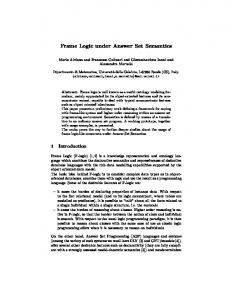
Fig. 1. The Lparse/Smodels System

Answer Sets

LPARSE

Ground Logic Program

Answer Set Program

Several efficient ASP solvers have been developed, such as Smodels (Niemelä and Simons 1997), DLV (Eiter et al. 1998), Cmodels (Giunchiglia et al. 2004), ASSAT (Lin and Zhao 2002), and CLASP (Gebser et al. 2007). One of the most popular ASP solvers is Smodels (Niemelä and Simons 1997; Simons et al. 2002) which comes with Lparse, a grounder. Lparse takes as input a logic program P and produces as output a simplified version of ground(P ). The output of Lparse is in turn accepted by Smodels, and used to produce the answer sets of P (see Figure 1).

8


The Lparse/Smodels system supports several extended types of literals, such as the cardinality literals, which are of the form: L {l1 , . . . , ln } U , where L and U are integers, L ≤ U , and l1 , . . . , ln are literals. The cardinality literal is satisfied by an answer set M if the number x of literals in {l1 , . . . , ln } that are true in M is such that L ≤ x ≤ U . The back-end engine, Smodels in Figure 1, produces the collection of answer sets of the input program. Various control options can be provided to guide the computation—e.g., establish a limit on the number of answer sets provided or request the answer set to contains specific atoms. We note that all of the available ASP solvers (Anger et al. 2005; Eiter et al. 1998; Gebser et al. 2007; Giunchiglia et al. 2004; Lin and Zhao 2002) operate in a similar fashion as Smodels. DLV uses its own grounder while others use Lparse. New grounder programs have also been recently proposed, e.g., Gringo in (Gebser et al. 2007). SAT-based answer set solvers rely on SAT-solver in computing answer sets (Giunchiglia et al. 2004; Lin and Zhao 2002). 3 Explanations The traditional methodology employed in ASP relies on encoding each problem Q as a logic program π(Q), whose answer sets are in one-to-one correspondence with the solutions of Q. From the software development perspective, it would be important to address the question “why is M an answer set of the program P ?” This question gives rise to the question “why does an atom a belong to M + (or M − )?” Answering this question can be very important, in that it provides us with explanations regarding the presence (or absence) of different atoms in M . Intuitively, we view answering these questions as the “declarative” parallel of answering questions of the type “why is 3.1415 the value of the variable x?” in the context of imperative languages—a question that can be typically answered by producing and analyzing an execution trace (or event trace (Auguston 2000)). The objective of this section is to develop the notion of explanation, as a graph structure used to describe the “reason” for the truth value of an atom w.r.t. a given answer set. In particular, each explanation graph will describe the derivation of the truth value (i.e., true or false) of an atom using the rules in the program. The explanation will also need to be flexible enough to explain those contradictory situations, arising during the construction of answer sets, where an atom is made true and false at the same time—for reference, these are the situations that trigger a backtracking in systems like Smodels (Simons et al. 2002). In the rest of this section, we will introduce this graph-based representation of the support for the truth values of atoms in an interpretation. In particular, we will incrementally develop this representation. We will start with a generic graph structure (Explanation Graph), which describes truth values without accounting for program rules. We will then identify specific graph patterns that can be derived from program rules (Local Consistent Explanations), and impose them on the explanation graph, to obtain the (J, A)-based Explanation Graphs. These graphs are used to explain the truth values of an atom w.r.t. an interpretation J and a set of


9

assumptions A—where an assumption is an atom for which we will not seek any explanations. The assumptions derive from the inherent “guessing” process involved in the definition of answer sets (and in their algorithmic construction), and they will be used to justify atoms that have been “guessed” in the construction of the answer set and for which a meaningful explanation cannot be constructed. Before we proceed, let us introduce notation that will be used in the following discussion. For an atom a, we write a+ to denote the fact that the atom a is true, and a− to denote the fact that a is false. We will call a+ and a− the annotated versions of a. Furthermore, we will define atom(a+ ) = a and atom(a− ) = a. For a set of atoms S, we define the following sets of annotated atoms: • S p = {a+ | a ∈ S}, • S n = {a− | a ∈ S}. Furthermore, we denote with not S the set not S = { not a | a ∈ S}. 3.1 Explanation Graphs In building the notion of justification, we will start from a very general (labeled, directed) graph structure, called explanation graph. We will incrementally construct the notion of justification, by progressively adding the necessary restrictions to it. Definition 3 (Explanation Graph) For a program P , an explanation graph (or e-graph) is a labeled, directed graph (N, E), where N ⊆ Ap ∪ An ∪ {assume, >, ⊥} and E ⊆ N × N × {+, −}, which satisfies the following properties: 1. 2. 3. 4.

the only sinks in the graph are: assume, >, and ⊥; for every b ∈ N ∩ Ap , we have that (b, assume, −) 6∈ E and (b, ⊥, −) 6∈ E; for every b ∈ N ∩ An , we have that (b, assume, +) 6∈ E and (b, >, +) 6∈ E; for every b ∈ N , if (b, l, s) ∈ E for some l ∈ {assume, >, ⊥} and s ∈ {+, −} then (b, l, s) is the only outgoing edge originating from b.

Property (1) indicates that each atom appearing in an e-graph should have outgoing edges (which will explain the truth value of the atom). Properties (2) and (3) ensure that true (false) atoms are not explained using explanations that are proper for false (true) atoms. Finally, property (4) ensures that atoms explained using the special explanations assume, >, ⊥ have only one explanation in the graph. Intuitively, • > will be employed to explain program facts—i.e., their truth does not depend on other atoms; • ⊥ will be used to explain atoms that do not have defining rules—i.e., the falsity is not dependent on other atoms; and • assume is used for atoms we are not seeking any explanations for. Each edge of the graph connects two annotated atoms or an annotated atom with one of the nodes in {>, ⊥, assume}, and it is marked by a label from {+, −}. Edges

10


labeled 0 +0 are called positive edges, while those labeled 0 −0 are called negative edges. A path in an e-graph is positive if it contains only positive edges, while a path is negative if it contains at least one negative edge. We will denote with (n1 , n2 ) ∈ E ∗,+ the fact that there is a positive path in the e-graph from n1 to n2 . Example 6 Figure 2 illustrates several simple e-graphs. Intuitively,

(i)

(ii)

(iii)

p+

p+

p-

q+ + assume

+

+

q+

r+

+

+

r+

T

-

-

sT

+

t-

assume

+

+

u-

+ T

Fig. 2. Simple e-graphs

• The graph (i) describes the true state of p by making it positively dependent on the true state of q and r; in turn, q is simply assumed to be true while r is a fact in the program. • The graph (ii) describes more complex dependencies; in particular, observe that t and u are both false and they are mutually dependent—as in the case of a program containing the rules t

:−

u.

u

:−

t.

Observe also that s is explained being false because there are no rules defining it. • The graph (iii) states that p has been simply assumed to be false. 2 Given an explanation graph and an atom, we can extract from the graph the elements that directly contribute to the truth value of the atom. We will call this set of elements the support of the atom. This is formally defined as follows. Definition 4 Let G = (N, E) be an e-graph and b ∈ N ∩ (Ap ∪ An ) a node in G. The direct support of b in G, denoted by support(b, G), is defined as follows. • support(b, G) = {atom(c) | (b, c, +) ∈ E} ∪ { not atom(c) | (b, c, −) ∈ E}, if for every ` ∈ {assume, >, ⊥} and s ∈ {+, −}, (b, `, s) 6∈ E; • support(b, G) = {`} if (b, `, s) ∈ E, ` ∈ {assume, >, ⊥} and s ∈ {+, −}.


11

Example 7 If we consider the e-graph (ii) in Figure 2, then we have that support(p+ , G2 ) = {q, not s, not t} while support(t− , G2 ) = {u}. We also have support(p+ , G1 ) = {q, r}. 2 It is worth mentioning that an explanation graph is a general concept aimed at providing arguments for answering the question ‘why is an atom true or false?’ In this sense, it is similar to the concept of a support graph used in program analysis (Saha and Ramakrishnan 2005). The main difference between these two concepts lies in that support graphs are defined only for definite programs while explanation graphs are defined for general logic programs. Furthermore, a support graph contains information about the support for all answer while an explanation graph stores only the support for one atom. An explanation graph can be used to answer the question of why an atom is false which is not the case for support graphs. 3.2 Local Explanations and (J, A)-based Explanations The next step towards the definition of the concept of justification requires enriching the general concept of e-graph with explanations of truth values of atoms that are derived from the rules of the program. A Local Consistent Explanation (LCE) describes one step of justification for a literal. Note that our notion of local consistent explanation is similar in spirit, but different in practice, from the analogous definition used in (Pemmasani et al. 2004; Roychoudhury et al. 2000). It describes the possible local reasons for the truth/falsity of a literal. If a is true, the explanation contains those bodies of the rules for a that are satisfied by I. If a is false, the explanation contains sets of literals that are false in I and they falsify all rules for a. The construction of a LCE is performed w.r.t. a possible interpretation and a set of atoms U —the latter contains atoms that are automatically assumed to be false, without the need of justifying them. The need for this last component (to be further elaborated later in the paper) derives from the practice of computing answer sets, where the truth value of certain atoms is first guessed and then later verified. Definition 5 (Local Consistent Explanation) Let P be a program, b be an atom, J a possible interpretation, U a set of atoms (assumptions), and S ⊆ A ∪ not A ∪ {assume, >, ⊥} a set of literals. We say that 1. S is a local consistent explanation of b+ w.r.t. (J, U ), if b ∈ J + and ◦ S = {assume}, or ◦ S ∩ A ⊆ J + , {c | not c ∈ S} ⊆ J − ∪ U , and there is a rule r in P such that head(r) = b and S = body(r); for convenience, we write S = {>} to denote the case where body(r) = ∅. 2. S is a local consistent explanation of b− w.r.t. (J, U ) if b ∈ J − ∪ U and

12

Enrico Pontelli, Tran Cao Son, and Omar Elkhatib ◦ S = {assume}; or ◦ S ∩ A ⊆ J − ∪ U , {c | not c ∈ S} ⊆ J + , and S is a minimal set of literals such that for every rule r ∈ P , if head(r) = b, then pos(r) ∩ S 6= ∅ or neg(r) ∩ {c | not c ∈ S} 6= ∅; for convenience, we write S = {⊥} to denote the case S = ∅.

We will denote with LCEPp (b, J, U ) the set of all the LCEs of b+ w.r.t. (J, U ), and with LCEPn (b, J, U ) the set of all the LCEs of b− w.r.t. (J, U ). Observe that U is the set of atoms that are assumed to be false. For this reason, negative LCEs are defined for elements J − ∪ U but positive LCEs are defined only for elements in J + . We illustrate this definition in a series of examples. Example 8 Let P be the program: p q

:− :−

q, r. r.

q. r.

The program admits only one answer set M = h{p, q, r}, ∅i. The LCEs for the atoms of this program w.r.t. (M, ∅) are: LCEPp (p, M, ∅) = {{q, r}, {assume}} LCEPp (q, M, ∅) = {{>}, {r}, {assume}} LCEPp (r, M, ∅) = {{>}, {assume}} 2 The above example shows a program with a unique answer set. The next example discusses the definition in a program with more than one answer set and an empty well-founded model. It also highlights the difference between the positive and negative LCEs for atoms given a partial interpretation and a set of assumptions. Example 9 Let P be the program: p

:−

not q.

q

:−

not p.

Let us consider the partial interpretation M = h{p}, ∅i. The following are LCEs w.r.t. (M, ∅): LCEPp (p, M, ∅) = {{assume}} LCEPn (q, M, ∅) = LCEPp (q, M, ∅) = {{⊥}} The above LCEs are explanations for the truth value of p and q being true and false with respect to M and the empty set of assumptions. Thus, the only explanation for p being true is that it is assumed to be true, since the only way to derive p to be true is to use the first rule and nothing is assumed to be false, i.e., not q is not true. On the other hand, q 6∈ M − ∪ ∅ leads to the fact that there is no explanation for q being false. Likewise, because q 6∈ M + , there is no positive LCE for q w.r.t. (M, ∅).


13

The LCEs w.r.t. (M, {q}) are: LCEPp (p, M, {q}) = {{assume}, { not q}} LCEPn (q, M, {q}) = {{assume}, { not p}} Assuming that q is false leads to one additional explanation for p being true. Furthermore, there are now two explanations for q being false. The first one is that it is assumed to be false and the second one satisfies the second condition in Definition 5. Consider the complete interpretation M 0 = h{p}, {q}i. The LCEs w.r.t. (M 0 , ∅) are: LCEPp (p, M 0 , ∅) = {{assume}, { not q}} LCEPn (q, M 0 , ∅) = {{assume}, { not p}} 2 The next example uses a program with a non-empty well-founded model. Example 10 Let P be the program: a f

:− :−

f, not b. e.

b d

:− :−

e, not a. c, e.

e. c

:−

d, f.

This program has the answer sets: M1 = h{f, e, b}, {a, c, d}i

M2 = h{f, e, a}, {c, b, d}i

Observe that the well-founded model of this program is hW + , W − i = h{e, f}, {c, d}i. The following are LCEs w.r.t. the answer set M1 and the empty set of assumptions (those for (M2 , ∅) have a similar structure): LCEPn (a, M1 , ∅) = {{ not b}, {assume}} LCEPp (b, M1 , ∅) = {{e, not a}, {assume}} LCEPp (e, M1 , ∅) = {{>}, {assume}} LCEPp (f, M1 , ∅) = {{e}, {assume}} LCEPn (d, M1 , ∅) = {{c}, {assume}} LCEPn (c, M1 , ∅) = {{d}, {assume}} 2 Let us open a brief parenthesis to discuss some complexity issues related to the existence of LCEs. First, checking whether or not there is a LCE of b+ w.r.t. (J, U ) is equivalent to checking whether or not the program contains a rule r whose head is b and whose body is satisfied by the interpretation hJ + , J − ∪ U i. This leads to the following observation. Observation 1 Given a program P , a possible interpretation J, a set of assumptions U , and an atom b, determining whether or not there is a LCE S of b+ w.r.t. (J, U ) such that S 6= {assume} can be done in time polynomial in the size of P . In order to determine whether or not there exists a LCE of b− w.r.t. (J, U ), we need to find a minimal set of literals S that satisfies the second condition of Definition

14


5. This can also be accomplished in time polynomial in the size of P . In fact, let Pb be the set of rules in P whose head is b. Furthermore, for a rule r, let Sr (J, U ) = {a | a ∈ pos(r) ∩ (J − ∪ U )} ∪ {not a | a ∈ J + ∩ neg(r)}. Intuitively, Sr (J, U ) is the maximal set of literals that falsifies the rule r w.r.t. (J, U ). To find a LCE for b− , it is necessary to have Sr (J, U ) 6= ∅ for every r ∈ Pb . Clearly, computing Sr (J, U ) for r ∈ Pb can be done in polynomial time in the size of P . Finding a minimal set S such that S ∩ Sr 6= ∅ for every r ∈ Pb can be done by scanning through the set Pb and adding to S (initially set to ∅) an arbitrary element of Sr (J, U ) if S ∩ Sr (J, U ) = ∅. This leads to the following observation. Observation 2 Given a program P , a possible interpretation J, a set of assumptions U , and an atom b, determining whether there exists a LCE S of b− w.r.t. (J, U ) such that S 6= {assume} can be done in time polynomial in the size of P . We are now ready to instantiate the notion of e-graph by forcing the edges of the e-graph to represent encodings of local consistent explanations of the corresponding atoms. To select an e-graph as an acceptable explanation, we need two additional components: the current interpretation (J) and the collection (U ) of elements that have been introduced in the interpretation without any “supporting evidence”. An e-graph based on (J, U ) is defined next. Definition 6 ((J, U )-Based Explanation Graph) Let P be a program, J a possible interpretation, U a set of atoms, and b an element in Ap ∪ An . A (J, U )-based explanation graph G = (N, E) of b is an e-graph such that • (Relevance) every node c ∈ N is reachable from b • (Correctness) for every c ∈ N \ {assume, >, ⊥}, support(c, G) is an LCE of c w.r.t. (J, U ) The two additional conditions we impose on the e-graph force the graph to be connected w.r.t. the element b we are justifying, and force the selected nodes and edges to reflect local consistent explanations for the various elements. The next condition we impose on the explanation graph is aimed at ensuring that no positive cycles are present. The intuition is that atoms that are true in an answer set should have a non-cyclic support for their truth values. Observe that the same does not happen for elements that are false—as in the case of elements belonging to unfounded sets (Apt and Bol 1994). Definition 7 (Safety) A (J, U )-based e-graph (N, E) is safe if ∀b+ ∈ N , (b+ , b+ ) 6∈ E ∗,+ .


15

Example 11 Consider the e-graphs in Figure 3, for the program of Example 10. Neither the e-graph of a+ ((i) nor the e-graph (ii)) is a (M1 , {c, d})-based e-graph of a+ , since support(b, G) = {assume} in both cases, and this does not represent a valid LCE for b− (since b ∈ / M1− ∪ {c, d}). Observe, on the other hand, that they are both acceptable (M2 , {b, c, d})-based e-graphs of a+ . The e-graph of c+ (the graph (iii)) is neither a (M1 , {c, d})-based nor a (M2 , {b, c, d})based e-graph of c+ , while the e-graph of c− (graph (iv)) is a (M1 , {c, d})-based and a (M2 , {b, c, d})-based e-graph of c− . Observe also that all the graphs are safe.

a+ -

a+ +

f+

b-

b-

+

assume

-

assume (i)

2

assume (ii)

c+ +

+ f+ + e+ +

d+ +

+

cf+ +

assume assume (iii)

+

+ d(iv)

Fig. 3. Sample (J, U )-based Explanation Graphs

4 Off-Line Justifications Off-line justifications are employed to characterize the “reason” for the truth value of an atom w.r.t. a given answer set M . The definition will represent a refinement of the (M, A)-based explanation graph, where A will be selected according to the properties of the answer set M . Off-line justifications will rely on the assumption that M is a complete interpretation. Let us start with a simple observation. If M is an answer set of a program P , and W FP is the well-founded model of P , then it is known that, W FP+ ⊆ M + and W FP− ⊆ M − (Apt and Bol 1994). Furthermore, we observe that the content of M is uniquely determined by the truth values assigned to the atoms in V = N AN T (P ) \ (W FP+ ∪ W FP− ), i.e., the atoms that • appear in negative literals in the program, and • their truth value is not determined by the well-founded model. We are interested in the subsets of V with the following property: if all the elements in the subset are assumed to be false, then the truth value of all other atoms in A is uniquely determined and leads to the desired answer set. We call these subsets the assumptions of the answer set. Let us characterize this concept more formally.

16


Definition 8 (Tentative Assumptions) Let P be a program and M be an answer set of P . The tentative assumptions of P w.r.t. M (denoted by T AP (M )) are defined as: T AP (M ) = {a | a ∈ N AN T (P ) ∧ a ∈ M − ∧ a 6∈ (W FP+ ∪ W FP− )} The negative reduct of a program P w.r.t. a set of atoms U is a program obtained from P by forcing all the atoms in U to be false. Definition 9 (Negative Reduct) Let P be a program, M an answer set of P , and U ⊆ T AP (M ) a set of tentative assumption atoms. The negative reduct of P w.r.t. U , denoted by N R(P, U ), is the set of rules: N R(P, U ) = P \ { r | head(r) ∈ U }. Example 12 Let us consider the program p :- not q. r :- p, s. s.

q :- not p. t :- q, u.

The well-founded model for this program is h{s}, {u}i. The program has two answer sets, M1 = h{p,s,r}, {t,u,q}i and M2 = h{q,s}, {p,r,t,u}i. The tentative assumptions for this program w.r.t. M1 is the set {q}. If we consider the set {q}, the negative reduct of the program is the set of rules p :- not q. r :- p, s. s.

t :- q, u. 2

We are now ready to introduce the proper concept of assumptions—these are those tentative assumptions that are sufficient to allow the reconstruction of the answer set. Definition 10 (Assumptions) Let P be a program and M be an answer set of P . An assumption w.r.t. M is a set of atoms U satisfying the following properties: (1) U ⊆ T AP (M ), and (2) the well-founded model of N R(P, U ) is equal to M —i.e., W FN R(P,U ) = M. We will denote with Assumptions(P, M ) the set of all assumptions of P w.r.t. M . A minimal assumption is an assumption that is minimal w.r.t. the set inclusion operator. We will denote with µAssumptions(P, M ) the set of all the minimal assumptions of P w.r.t. M . An important observation we can make is that Assumptions(P, M ) is not an empty set, since the complete set T AP (M ) is an assumption.


17

Proposition 1 Given a program P and an answer set M of P , the well-founded model of the program N R(P, T AP (M )) is equal to M . Proof Appendix A. Example 13 Let us consider the program of Example 9. The interpretation M = h{p}, {q}i is an answer set. For this program we have: W FP = T AP (h{p}, {q}i) =

h∅, ∅i {q}

Observe that N R(P, {q}) = {p :− not q}. The well-founded model of this program is h{p}, {q}i, which is equal to M . Thus, {q} is an assumption of P w.r.t. M . In particular, one can see that this is the only assumption we can have. 2 Example 14 Let us consider the following program P : a f k

:− :− :−

f, not b. e. a.

b d

:− :−

e, not a. c, e.

e. c

:−

d, f, not k.

The interpretation M1 = h{f, e, b}, {a, c, d, k}i is an answer set of the program. In particular: W FP T AP (h{f, e, b}, {a, c, d}i)

= h{e, f}, {d, c}i = {a, k}

The program N R(P, {a}) is: b f c

:− :− :−

e, not a. e. d, f, not k.

e. d k

:− :−

c, e. a.

The well-founded model of this program is h{e, f, b}, {a, c, d, k}i. Thus, {a} is an assumption w.r.t. M1 . Observe also that if we consider N R(P, {a, k}) b f c

:− :− :−

e, not a. e. d, f, not k.

e. d

:−

c, e.

The well-founded model of this program is also h{e, f, b}, {a, c, d, k}i, thus making {a, k} another assumption. Note that this second assumption is not minimal. 2 We will now specialize e-graphs to the case of answer sets, where only false elements can be used as assumptions.

18


Definition 11 (Off-line Explanation Graph) Let P be a program, J a partial interpretation, U a set of atoms, and b an element in Ap ∪ An . An off-line explanation graph G = (N, E) of b w.r.t. J and U is a (J, U )-based e-graph of b satisfying the following additional conditions: ◦ there exists no p+ ∈ N such that (p+ , assume, +) ∈ E; and ◦ (p− , assume, −) ∈ E iff p ∈ U . We will denote with E(b, J, U ) the set of all off-line explanation graphs of b w.r.t. J and U . The first condition ensures that true elements cannot be treated as assumptions, while the second condition ensures that only assumptions are justified as such in the graph. Definition 12 (Off-line Justification) Let P be a program, M an answer set, U ∈ Assumptions(P, M ), and a ∈ Ap ∪ An . An off-line justification of a w.r.t. M and U is an element (N, E) of E(a, M, U ) which is safe. If M is an answer set and x ∈ M + (resp. x ∈ M − ), then G is an off-line justification of x w.r.t. M and the assumption U iff G is an off-line justification of x+ (resp. x− ) w.r.t. M and U . Example 15 Let us consider the program in Example 10. We have that N AN T (P ) = {b, a}. The assumptions for this program are: Assumptions(P, M1 ) = {{a}}

and

Assumptions(P, M2 ) = {{b}}.

The off-line justifications for atoms in M1 w.r.t. M1 and {a} are shown in Figure 4. b+ a-

f+ +

+ e+ +

e+ +

e+ +

c+

+ d-

aassume

assume

Fig. 4. Off-line justifications w.r.t. M1 and {a} for b+ , f + , e+ , c− and a− (left to right)

Justifications are built by assembling items from the LCEs of the various atoms and avoiding the creation of positive cycles in the justification of true atoms. Also, the justification is built w.r.t. a chosen set of assumptions (A), whose elements are all assumed false. In general, an atom may admit multiple justifications, even w.r.t. the same assumptions. The following lemma shows that elements in W FP can be justified without negative cycles and assumptions.


19

Lemma 4.1 Let P be a program, M an answer set, and W FP the well-founded model of P . Each atom a ∈ W FP has a justification w.r.t. M and ∅ which does not contain any negative cycle. From the definition of assumption and from the previous lemma we can infer that a justification free of negative cycles can be built for every atom. Proposition 2 Let P be a program and M an answer set. For each atom a, there is an off-line justification w.r.t. M and M − \ W FP− which does not contain negative cycles. Proposition 2 underlines an important property—the fact that all true elements can be justified in a non-cyclic fashion. This makes the justification more natural, reflecting the non-cyclic process employed in constructing the minimal answer set (e.g., using the iterations of TP ) and the well-founded model (e.g., using the characterization in (Brass et al. 2001)). This also gracefully extends a similar property satisfied by the justifications under well-founded semantics used in (Roychoudhury et al. 2000). Note that the only cycles possibly present in the justifications are positive cycles associated to (mutually dependent) false elements—this is an unavoidable situation due the semantic characterization in well-founded and answer set semantics (e.g., unfounded sets). A similar design choice has been made in (Pemmasani et al. 2004; Roychoudhury et al. 2000). Example 16 Let us reconsider the following program P from Example 14: a f k

:− :− :−

f, not b. e. a.

b d

:− :−

e, not a. c, e.

e. c

:−

d, f, not k.

and the answer set M = h{f, e, b}, {a, c, d, k}i is an answer set of the program. The well-founded model of this program is W FP = h{e, f}, {d, c}i a and k are assumed to be false. Off-line justifications for b+ , f+ , e+ and for c− , d− , a− with respect to M and M − \ W FP− = {a, k}, which do not contain negative cycles, are the same as those depicted in Figure 4. k− has an off-line justification in which it is connected to assume by a negative edge, as it is assumed to be false. 2 5 On-Line Justifications for ASP Off-line justifications provide a “declarative trace” for the truth values of the atoms present in an answer set. The majority of the inference engines for ASP construct answer sets in an incremental fashion, making choices (and possibly undoing them) and declaratively applying the rules in the program. Unexpected results (e.g., failure to produce any answer sets) require a more refined view of computation. One way

20


to address this problem is to refine the notion of justification to make possible the “declarative tracing” of atoms w.r.t. a partially constructed interpretation. This is similar to debugging of imperative languages, where breakpoints can be set and the state of the execution explored at any point during the computation. In this section, we introduce the concept of on-line justification, which is generated during the computation of an answer set and allows us to justify atoms w.r.t. an incomplete interpretation—that represents an intermediate step in the construction of the answer set. 5.1 Computation The concept of on-line justification is applicable to computation models that construct answer sets in an incremental fashion, e.g., Smodels and DLV (Simons et al. 2002; Eiter et al. 1998; Gebser et al. 2007; Anger et al. 2005). We can view the computation as a sequence of steps, each associated to a partial interpretation. We will focus, in particular, on computation models where the progress towards the answer set is monotonic. Definition 13 (General Computation) Let P be a program. A general computation is a sequence M0 , M1 , . . . , Mk , such that (i) M0 = h∅, ∅i, (ii) M0 , . . . , Mk−1 are partial interpretations, and (iii) Mi v Mi+1 for i = 0, . . . , k − 1. A general complete computation is a computation M0 , . . . , Mk such that Mk is an answer set of P . In general, we do not require Mk —the ending point of the computation—to be a partial interpretation, since we wish to model computations that can also “fail”— i.e., Mk+ ∩ Mk− 6= ∅. This is, for example, what might happen during a Smodels computation—whenever the Conflict function succeeds (Simons et al. 2002). We will refer to a pair of sets of atoms as a possible interpretation (or p-interpretation for short). Clearly, each partial interpretation is a p-interpretation, but not vice versa. Abusing the notation, we use J + and J − to indicate the first and second component of a p-interpretation J; moreover, I v J denotes that I + ⊆ J + and I − ⊆ J −. Our objective is to associate a form of justification to each intermediate step Mi of a general computation. Ideally, we would like the justifications associated to each Mi to explain truth values in the “same way” as in the final off-line justification. Since the computation model might rely on guessing some truth values, Mi might not contain sufficient information to develop a valid justification for each element in Mi . We will identify those atoms for which a justification can be constructed given Mi . These atoms describe a p-interpretation Di v Mi . The computation of Di is defined based on the two operators, Γ and ∆, which will respectively compute Di+ and Di− .


21

Let us start with some preliminary definitions. Let P be a program and I be a p-interpretation. A set of atoms S is called a cycle w.r.t. I if, for every a ∈ S and for each r ∈ P such that head(r) = a, we have that one of the following holds: • pos(r) ∩ I − 6= ∅ (rule is falsified by I), or • neg(r) ∩ I + 6= ∅ (rule is falsified by I), or • pos(r) ∩ S 6= ∅ (rule is in a cycle with elements of S). We can observe that, if I is an interpretation, S is a cycle w.r.t. I, and M is an answer set with I v M , then S ⊆ M − —since the elements of S are either falsified by the interpretation (and, thus, by M ) or they are part of an unfounded set. The set of cycles w.r.t. I is denoted by cycles(I). Furthermore, for every element a ∈ Ap ∪ An , let P E(a, I) be the set of local consistent explanations of a w.r.t. I and ∅—i.e., LCEs that do not require any assumptions and that build on the interpretation I. We are now ready to define the operators that will compute the Di subset of the p-interpretation Mi . Definition 14 Let P be a program and I v J be two p-interpretations. We define ΓI (J) = ∆I (J) =

I + ∪ {head(r) ∈ J + | r ∈ P, I |= body(r)} S I − ∪ {a ∈ J − | P E(a− , I) 6= ∅} ∪ {S | S ∈ cycles(I), S ⊆ J − }

Intuitively, for I v J, ΓI (J) is a set of atoms that are true in J and they will remain true in every answer set extending J, if J is a partial interpretation. The set ∆I (J) contains atoms that are false in J and in each answer set that extends J. In particular, if I is the set of “justifiable” atoms—i.e., atoms for which we can construct a justification—and J is the result of the current computation step, then we have that hΓI (J), ∆I (J)i is a new interpretation satisfying the following two properties: • I v hΓI (J), ∆I (J)i v J, and • it is possible to create a justification for all elements in hΓI (J), ∆I (J)i. Observe that it is not necessarily true that ΓI (J) = J + and ∆I (J) = J − . This means that there may be elements in the current step of computation for which it is not possible (yet) to construct a justification. This reflects the practice of guessing literals and propagating these guesses in the computation of answer sets, implemented by several solvers (based on variations of the Davis-Putnam-LogemannLoveland procedure (Davis et al. 1962)). We are now ready to specify how the set Di is computed. Let W FP = hW + , W − i be the well-founded model of P and let J be a p-interpretation.2 Γ0 (J) = Γh∅,∅i (J) Γi+1 (J) = ΓIi (J) (where Ii = hΓi (J), ∆i (J)i) 2

∆0 (J) = T AP (J) ∪ ∆h∅,∅i (J) ∆i+1 (J) = ∆Ii (J)

Remember that T AP (J) = {a | a ∈ N AN T (P ) ∧ a ∈ J − ∧ a 6∈ (W FP+ ∪ W FP− )}.

22


Intuitively, 1. The iteration process starts by collecting the facts of P (Γ0 ) and all those elements that are false either because there are no defining rules for them or because they have been chosen to be false in the construction of J. All these elements can be easily provided with justifications. 2. The successive iterations expand the set of known justifiable elements from J using Γ and ∆. Finally, we repeat the iteration process until a fixpoint is reached: Γ(J) =

∞ [

Γi (J)

and

∆(J) =

i=0 i

i+1

∞ [

∆i (J)

i=0 +

i

i+1

Because Γ (J) ⊆ Γ (J) ⊆ J and ∆ (J) ⊆ ∆ (J) ⊆ J − (recall that I v J), we know that both Γ(J) and ∆(J) are well-defined. We can prove the following: Proposition 3 For a program P , we have that: • Γ and ∆ maintains the consistency of J, i.e., if J is an interpretation, then hΓ(J), ∆(J)i is also an interpretation; • Γ and ∆ are monotone w.r.t the argument J, i.e., if J v J 0 then Γ(J) ⊆ Γ(J 0 ) and ∆(J) ⊆ ∆(J 0 ); • Γ(W FP ) = W FP+ and ∆(W FP ) = W FP− ; and • If M is an answer set of P , then Γ(M ) = M + and ∆(M ) = M − . We next introduce the notion of on-line explanation graph. Definition 15 (On-line Explanation Graph) Let P be a program, A a set of atoms, J a p-interpretation, and a ∈ Ap ∪ An . An on-line explanation graph G = (N, E) of a w.r.t. J and A is a (J, A)-based e-graph of a. In particular, if J is an answer set of P , then any off-line e-graph of a w.r.t. J and A is also an on-line e-graph of a w.r.t. J and A. Observe that Γ0 (J) contains the set of facts of P that belongs to J + , while ∆0 (J) contains the set of atoms without defining rules and atoms belonging to positive cycles of P . As such, it is easy to see that, for each atom a in hΓ0 (J), ∆0 (J)i, we can construct an e-graph for a+ or a− whose nodes belong to Γ0 (J) ∪ ∆0 (J). Moreover: • if a ∈ Γi+1 (J) \ Γi (J), then an e-graph with nodes (except a+ ) belonging to Γi (J) ∪ ∆i (J) can be constructed; • if a ∈ ∆i+1 (J) \ ∆i (J), an e-graph with nodes (except a− ) belonging to Γi+1 (J) ∪ ∆i+1 (J) can be constructed. This leads to the following lemma.


23

Lemma 5.1 Let P be a program, J a p-interpretation, and A = T AP (J). The following properties hold: • For each atom a ∈ Γ(J) (resp. a ∈ ∆(J)), there exists a safe off-line e-graph of a+ (resp. a− ) w.r.t. J and A; • for each atom a ∈ J + \ Γ(J) (resp. a ∈ J − \ ∆(J)) there exists an on-line e-graph of a+ (resp. a− ) w.r.t. J and A. We will now discuss how the above proposition can be utilized in defining a notion called on-line justification. To this end, we associate to each partial interpretation J a snapshot S(J): Definition 16 A snapshot of a p-interpretation J is a tuple S(J) = hOff(J), On(J), Di, where • D = hΓ(J), ∆(J)i, • For each a in Γ(J), Off(J) contains exactly one safe off-line e-graph of a+ w.r.t. J and T AP (J); • For each a in ∆(J), Off(J) contains exactly one safe off-line e-graph of a− w.r.t. J and T AP (J); • For each a ∈ J + \ Γ(J), On(J) contains exactly one on-line e-graph of a+ w.r.t. J and T AP (J); • For each a ∈ J − \ ∆(J), On(J) contains exactly one on-line e-graph of a− w.r.t. J and T AP (J). Definition 17 (On-line Justification) Given a computation M0 , M1 , . . . , Mk , an on-line justification of the computation is a sequence of snapshots S(M0 ), S(M1 ), . . . , S(Mk ). It is worth to point out that an on-line justification can be obtained in answer set solvers employing the computation model described in Definition 13. This will be demonstrated in the next section where we discuss the computation of on-line justifications in the Smodels system. We next illustrate the concept of an on-line justification. Example 17 Let us consider the program P containing s e.

:−

a, not t.

a f

:− :−

f, not b. e.

b

:−

e, not a.

Two possible general computations of P are M01 = h{e, s}, ∅i M02 = h{e, f}, ∅i

7→ 7→

M11 = h{e, s, a}, {t}i M12 = h{e, f}, {t}i

7→ 7→

M21 = h{e, s, a, f}, {t, b}i M22 = h{e, f, b, a}, {t, a, b, s}i

The first computation is a complete computation leading to an answer set of P while the second one is not.

24

Enrico Pontelli, Tran Cao Son, and Omar Elkhatib An on-line justification for the first computation is given next: S(M01 ) = hX0 , Y0 , h{e}, ∅ii S(M11 ) = hX0 ∪ X1 , Y0 ∪ Y1 , h{e}, {t}ii S(M12 ) = hX0 ∪ X1 ∪ X2 , ∅, M21 i

where (for the sake of simplicity we report only the edges of the graphs): X0 Y0 X1 Y1 X2

= = = = =

{(e+ , >, +)} {(s+ , assume, +)} {(t− , ⊥, −)} {(a+ , assume, +)} {(f+ , e+ , +), (s+ , a+ , +), (s+ , t− , −), (a+ , f+ , +), (a+ , b− , −), (b− , assume, −)}

An on-line justification for the second computation is: S(M02 ) = S(M12 ) = S(M22 ) =

hX0 , Y0 , h{e, f}, ∅ii hX0 ∪ X1 , Y0 , h{e, f}, {t}ii hX0 ∪ X1 ∪ X2 , Y0 ∪ Y2 , M22 i

where: X0 Y0 X1 Y1 X2 Y2

= = = = = =

{(e+ , >, +), (f+ , e+ , +)} ∅ {(t− , ⊥, −)} ∅ {(a+ , f+ , +), (a+ , b− , −), (b+ , e+ , +), (b+ , a− , −)} {(a− , assume, −), (b− , assume, −)} 2

We can relate the on-line justifications and off-line justifications as follows. Lemma 5.2 Let P be a program, J an interpretation, and M an answer set such that J v M . For every atom a, if (N, E) is a safe off-line e-graph of a w.r.t. J and A where A = J − ∩ T AP (M ) then it is an off-line justification of a w.r.t. M and T AP (M ). This leads to the following proposition. Proposition 4 Let M0 , . . . , Mk be a general complete computation and S(M0 ), . . . , S(Mk ) be an on-line justification of the computation. Then, for each atom a in Mk , the e-graph of a in S(Mk ) is an off-line justification of a w.r.t. Mk and T AP (Mk ). 6 Smodels On-line Justifications The notion of on-line justification presented in the previous section is very general, to fit the needs of different answer set solver implementations that follow the computation model presented in Subsection 5.1. In this section, we illustrate how the notion of on-line justification has been specialized to (and implemented in) a specific computation model—the one used in Smodels (Simons et al. 2002). This


25

allows us to define an incremental version of on-line justification—where the specific steps performed by Smodels are used to guide the incremental construction of the justification. The choice of Smodels was dictated by availability of its source code and its elegant design. We begin with an overview of the algorithms employed by Smodels. The following description has been adapted from (Giunchiglia and Maratea 2005; Simons et al. 2002). Although more abstract than the concrete implementation, and without various implemented features (e.g., heuristics, lookahead), it is sufficiently faithful to capture the spirit of our approach, and to guide the implementation (see Section 6.3). 6.1 An Overview of Smodels’ Computation We propose a description of the Smodels algorithms based on a composition of state-transformation operators. In the following, we say that an interpretation I does not satisfy the body of a rule r (i.e., body(r) is false in I) if (pos(r) ∩ I − ) ∪ (neg(r) ∩ I + ) 6= ∅. AtLeast Operator: The AtLeast operator is used to expand a partial interpretation I in such a way that each answer set M of P that “agrees” with I—i.e., the elements in I have the same truth value in M (or I v M )—also agrees with the expanded interpretation. Given a program P and a partial interpretation I, we define the intermediate operators AL1P , . . . , AL4P as follows: • Case 1. if r ∈ P , head(r) ∈ / I + , pos(P ) ⊆ I + and neg(P ) ⊆ I − then AL1P (I)+ = I + ∪ {head(r)}

and

AL1P (I)− = I −

• Case 2. if a ∈ / I + ∪ I − and ∀r ∈ P.(head(r) = a ⇒ body(r) is false in I), then AL2P (I)+ = I +

and

AL2P (I)− = I − ∪ {a}

• Case 3. if a ∈ I + and r is the only rule in P with head(r) = a and whose body is not false in I then AL3P (I)+ = I + ∪ pos(r) and AL3P (I)− = I − ∪ neg(r) • Case 4. if a ∈ I − , head(r) = a, and — if pos(r) \ I + = {b} then AL4P (I)+ = I + and AL4P (I)− = I − ∪ {b} — if neg(r) \ I + = {b} then AL4P (I)+ = I + ∪ {b} and AL4P (I)− = I − Given a program P and an interpretation I, ALP (I) = ALiP (I) if ALiP (I) 6= I and ∀j < i. ALjP (I) = I (1 ≤ i ≤ 4); otherwise, ALP (I) = I.

26

Enrico Pontelli, Tran Cao Son, and Omar Elkhatib AtMost Operator:

The AtM ostP operator recognizes atoms that are defined exclusively as mutual positive dependences (i.e., “positive loops”)—and falsifies them. Given a set of atoms S, the operator AMP is defined as AMP (S) = S ∪{head(r)|r ∈ P ∧pos(r) ⊆ S}. Given an interpretation I, the AtM ostP (I) operator is defined as [ AtM ostP (I)+ = I + and AtM ostP (I)− = I − ∪ {p ∈ A | p 6∈ Si } i≥0

where S0 = I + and Si+1 = AMP (Si ). Choose Operator: This operator is used to randomly select an atom that is unknown in a given interpretation. Given a partial interpretation I, chooseP returns an atom of A such that chooseP (I) 6∈ I + ∪ I −

and chooseP (I) ∈ N AN T (P ) \ (W FP+ ∪ W FP− ). Smodels Computation:

Given an interpretation I, we define the transitions: £ I 7→ALc I0 If I 0 = ALcP (I), c ∈ {1, 2, 3, 4} I

7→atmost

I0

I

7→choice

I0

£ ·

If I 0 = AtM ostP (I) If I 0 = hI + ∪ {chooseP (I)}, I − i or I 0 = hI + , I − ∪ {chooseP (I)}i

If there is an α in {AL1 , AL2 , AL3 , AL4 , atmost, choice} such that I 7→α I 0 , then we will simply denote this fact with I 7→ I 0 . function smodels(P ): S = h∅, ∅i; loop S = expand(P , S); if (S + ∩ S − 6= ∅) then fail; if (S + ∪ S − = A) then success(S); pick either% non-deterministic choice S + = S + ∪ {choose(S)} or S − = S − ∪ {choose(S)} endloop;

Fig. 5. Sketch of smodels

function expand(P , S): loop S 0 = S; repeat S = ALP (S); until (S = ALP (S)); S = AtM ost(P , S); if (S 0 = S) then return (S); endloop;

Fig. 6. Sketch of expand

The Smodels system imposes constraints on the order of application of the


27

transitions. Intuitively, the Smodels computation is depicted in the algorithms of Figs. 5 and 6. We will need the following notations. A computation I0 7→ I1 7→ I2 7→ . . . 7→ In is said to be AL-pure if every transition in the computation is an ALc transitions and for every c ∈ {1, 2, 3, 4}, ALcP (In ) = In . A choice point of a computation I0 7→ I1 7→ I2 7→ . . . 7→ In is an index 1 ≤ j < n such that Ij 7→choice Ij+1 . Definition 18 (Smodels Computation) Let P be a program. Let C = I0 7→ I1 7→ I2 7→ . . . 7→ In be a computation and 0 ≤ ν1 < ν2 < · · · < νr < n (r ≥ 0) be the sequence of all choice points in C. We say that C is a Smodels computation if for every 0 ≤ j ≤ r, there exists a sequence of indices νj + 1 = a1 < a2 < . . . < at ≤ νj+1 − 1 (νr+1 = n and ν0 = −1) such that • the transition Iai+1 −1 7→ Iai+1 is an 7→atmost transition (1 ≤ i ≤ t − 1) • the computation Iai 7→ . . . 7→ Iai+1 −1 is a AL-pure computation. We illustrate this definition in the next example. Example 18 Consider the program of Example 10. A possible computation of M1 is:3 h∅, ∅i 7→AL1 h{e, f}, {c, d}i 7→choice

h{e}, ∅i 7→AL1 h{e, f, b}, {c, d}i 7→AL2

h{e, f}, ∅i 7→atmost h{e, f, b}, {c, d, a}i 2

6.2 Smodels On-line Justifications We can use knowledge of the specific steps performed by Smodels to guide the construction of an on-line justification. Assuming that C = M0 7→ M1 7→ M2 7→ . . . 7→ Mn is a computation of Smodels. Let S(Mi ) = hE1 , E2 , Di and S(Mi+1 ) = hE10 , E20 , D0 i be the snapshots correspond to Mi and Mi+1 respectively. Obviously, S(Mi+1 ) can be computed by the following steps: • computing D0 = hΓ(Mi+1 ), ∆(Mi+1 )i; • updating E1 and E2 to obtain E10 and E20 . We observe that hΓ(Mi+1 ), ∆(Mi+1 i can be obtained by computing the fixpoint of the Γ- and ∆-function with the starting value ΓhΓ(Mi ),∆(Mi )i and ∆hΓ(Mi ),∆(Mi )i . This is possible due to the monotonicity of the computation. Regarding E10 and E20 , 3

We omit the steps that do not change the interpretation.

28


observe that the e-graphs for elements in hΓk (Mi+1 ), ∆k (Mi+1 )i can be constructed using the e-graphs constructed for elements in hΓk−1 (Mi+1 ), ∆k−1 (Mi+1 )i and the rules involved in the computation of hΓk (Mi+1 ), ∆k (Mi+1 )i. Thus, we only need to update E10 with e-graphs of elements of hΓk (Mi+1 ), ∆k (Mi+1 )i which do not belong to hΓk−1 (Mi+1 ), ∆k−1 (Mi+1 )i. Also, E20 is obtained from E2 by removing the e-graphs of atoms that “move” into D0 and adding the e-graph (a, assume, +) + − (resp. (a, assume, −)) for a ∈ Mi+1 (resp. a ∈ Mi+1 ) not belonging to D0 . Clearly, this computation depends on the transition from Mi to Mi+1 . Assume that Mi 7→α Mi+1 , the update of S(Mi ) to create S(Mi+1 ) is done as follows. • α ≡ choice: let p be the atom chosen in this step. If p is chosen to be true, then we can use the graph Gp = ({a, assume}, {(a, assume, +)}) and the resulting snapshot is S(Mi+1 ) = hE1 , E2 ∪ {Gp }, Di. Observe that D is unchanged, since the structure of the computation (in particular the fact that an expand has been done before the choice) ensures that p will not appear in the computation of D. If p is chosen to be false, then we will need to add p to D− , compute Γ(Mi+1 ) and ∆(Mi+1 ), and update E1 and E2 correspondingly; in particular, p belongs to ∆(Mi+1 ) and Gp = ({a, assume}, {(a, assume, −)}) is added to E1 . • α ≡ atmost: in this case, Mi+1 = hMi+ , Mi− ∪ AtM ost(P, Mi )i. The computation of S(Mi+1 ) is performed as from definition of on-line justification. In particular, observe that if ∀c ∈ AtM ost(P, Mi ) we have that LCEPn (c, D) 6= ∅ then the computation can be started from Γ(Mi ) and ∆(Mi )∪AtM ost(P, Mi ). • α ≡ AL1 : let p be the atom dealt with in this step and let r be the rule employed. We have that Mi+1 = hMi+ ∪ {p}, Mi− i. If D |= body(r) then S(Mi+1 ) will be computed starting from Γ(Mi )∪{p} and ∆(Mi ). In particular, an off-line graph for p, let’s say Gp , will be added to E1 , and such graph will be constructed using the LCE based on the rule r and the e-graphs in E1 . Otherwise, S(Mi+1 ) = hE1 , E2 ∪ {G+ (p, r, Σ)}, Di, where G+ (p, r, Σ) is an e-graph of p+ constructed using the LCE of rule r and the e-graphs in Σ = E1 ∪ E2 (note that all elements in body(r) have an e-graph in E1 ∪ E2 ). • α ≡ AL2 : let p be the atom dealt with in this step. In this case Mi+1 = hMi+ , Mi− ∪ {p}i. If there exists γ ∈ LCEPn (p, D, ∅), then S(Mi+1 ) can be computed according to the definition of on-line justification, starting from Γ(Mi ) and ∆(Mi ) ∪ {p}. Observe that the graph of p can be constructed starting with {(p, a, +) | a ∈ γ} ∪ {(p, b, −) | not b ∈ γ}). Otherwise, given an arbitrary ψ ∈ LCEPn (p, Mi , ∅), we can construct an egraph Gp for p− , such that ψ = support(p− , Gp ), the graphs E1 ∪ E2 are used to describe the elements of ψ, and S(Mi+1 ) = hE1 , E2 ∪ {Gp }, Di. • α ≡ AL3 : let r be the rule used in this step and let p = head(r). Then Mi+1 = hMi+ ∪ pos(r), Mi− ∪ neg(r)i and S(Mi+1 ) is computed according to the definition of on-line justification. Observe that the e-graph Gp for p+ (added to E1 or E2 ) for S(Mi+1 ) will be constructed using body(r) as


29

support(p+ , Gp ), and using the e-graphs in E1 ∪ E2 ∪ Σ for some Σ ⊆ {(a+ , assume, +) | a ∈ pos(r)} ∪ {(a, assume, −) | a ∈ neg(r)}. • α ≡ AL4 : let r be the rule processed and let b the atom detected in the body. If b ∈ pos(r), then Mi+1 = hMi+ , Mi− ∪ {b}i, while if b ∈ neg(r) then Mi+1 = hMi+ ∪ {b}, Mi− i. In either cases, the snapshot S(Mi+1 ) will be computed using the definition of on-line justification.

Example 19 Let us consider the computation of Example 18. A sequence of snapshots is (we provide only the edges of the graphs and we combine together e-graphs of different atoms):

S(M0 ) S(M1 ) S(M2 ) S(M3 ) S(M4 )

S(M5 )

E1

E2

D

∅ {(e+ , >, +)} {(e+ , >, +), (f + , e+ , +)} ½ + ¾ (e , >, +), {f + , e+ , +) (d− , c− , +), (c− , d− , +) ½ + ¾ (e , >, +), {f + , e+ , +) (d− , c− , +), (c− , d− , +)  +  (e , >, +), {f + , e+ , +),      − −  (d , c , +), (c− , d− , +), −   (a , assume, −),     (b+ , e+ , +), (b+ , a− , −)

∅ ∅ ∅

∅ h{e}, ∅i h{e, f }, ∅i

∅

h{e, f }, {c, d}i

{(b+ , assume, +)}

h{e, f }, {c, d}i

∅

h{e, f, b}, {c, d, a}i

2

Example 20 Let P be the program: p r

:− :−

not q not p

q p

:− :−

not p r

This program does not admit any answer sets where p is false. One possible computation (we highlight only steps that change the trace): 1. 3.

h∅, ∅i 7→choice h{q}, {p}i 7→AL1

2. h∅, {p}i 7 AL1 → 4. h{q, r}, {p}i → 7 AL1

5.

From this computation we can obtain a sequence of snapshots:

h{q, r, p}, {p}i

30


S(M0 ) S(M1 ) S(M2 ) S(M3 ) S(M4 )

E1

E2

D

∅ {(p− , assume, −)} {(p− , assume, −), (q + , p− , −)} − {(p , assume, −), (q + , p− , −), (r+ , p− , −)} ¾ ½ − (p , assume, −), (q + , p− , −), (r+ , p− , −), (p+ , r+ , +)

∅ ∅ ∅ ∅

∅ h∅, {p}i i h{q}, {p}i h{q, r}, {p}i

∅

h{p, q, r}, {p}i

Observe that a conflict is detected by the computation and the sources of conflict are highlighted in the presence of two justifications for p, one for p+ and another one for p− . 2 6.3 Discussion In this subsection, we discuss possible ways to extend the notion of justifications on various language extensions of ASP. We also describe a system capable of computing off-line and on-line justifications for ASP programs. 6.3.1 Language Extensions In the discussion presented above, we relied on a standard logic programming language. Various systems, such as Smodels, have introduced language extensions, such as choice atoms, to facilitate program development. The extension of the notion of justification to address these extensions is relatively straightforward. Let us consider, for example, the choice atom construct of Smodels. A choice atom has the form L ≤ {a1 , . . . , an , not b1 , . . . , not bm } ≤ U where L, U are integers (with L ≤ U ) and the various ai , bj are atoms. Choice atoms are allowed to appear both in the head as well as the body of rules. Given an interpretation I and a choice atom, we say that I satisfies the atom if L ≤ |{ai | ai ∈ I + }| + |{bj | bj ∈ I − }| ≤ U The local consistent explanation of a choice atom can be developed in a natural way: • If the choice atom L ≤ T ≤ U is true, then a set of literals S is an LCE if — A ∩ S ⊆ T and not A ∩ S ⊆ T — for each S 0 such that S ⊆ S 0 and {atom(`) | ` ∈ S 0 } = {atom(`) | ` ∈ T } we have that L ≤ |{a | a ∈ T ∩ A ∩ S 0 }| + |{b | not b ∈ T ∩ S 0 }| ≤ U • if the choice atom L ≤ T ≤ U is false, then a set of literals S is an LCE if


31

— A ∩ S ⊆ T and not A ∩ S ⊆ T — for each S 0 such that S ⊆ S 0 and {atom(`) | ` ∈ S 0 } = {atom(`) | ` ∈ T } we have that L > |{a | a ∈ T ∩ A ∩ S 0 }| + |{b | not b ∈ T ∩ S 0 }| or |{a | a ∈ T ∩ A ∩ S 0 }| + |{b | not b ∈ T ∩ S 0 }| > U The notions of e-graphs can be extended to include choice atoms. Choice atoms in the body are treated as such and justified according to the new notion of LCE. On the other hand, if we have a rule of the type L ≤ T ≤ U :− Body and M is an answer set, then we will • treat the head as a new (non-choice) atom (newL≤T ≤U ), and allow its justification in the usual manner, using the body of the rule • for each atom p ∈ T ∩ M + , the element p+ has a new LCE {newL≤T ≤U } Example 21 Consider the program containing the rules: p :− 2 ≤ {r,t,s} ≤ 2

q :−

:−

p, q

The interpretation h{t, s, p, q}, {r}i is an answer set of this program. The off-line justifications for s+ and t+ are illustrated in Figure 7. 2 The concept can be easily extended to deal with weight atoms.

t+

+

+

2{r,s,t}2

q+ +

p+ + T

T

+

+

+

assume

+ q+ + T

2{r,s,t}2

p+

-

new +

new + +

r-

s+

T

Fig. 7. Justifications in presence of choice atoms

32

Enrico Pontelli, Tran Cao Son, and Omar Elkhatib 6.3.2 Concrete Implementation

The notions of off-line and on-line justifications proposed in the previous sections have been implemented and integrated in a debugging system for Answer Set Programming, developed within the ASP − PROLOG framework (Elkhatib et al. 2004). The notions of justification proposed here is meant to represent the basic data structure on which debugging strategies for ASP can be developed. ASP − PROLOG allows the construction of Prolog programs—using CIAO Prolog (Gras and Hermenegildo 2000)—which include modules written in ASP (the Smodels flavor of ASP). In this sense, the embedding of ASP within a Prolog framework (as possible in ASP − PROLOG) allows the programmer to use Prolog itself to query the justifications and develop debugging strategies. We will begin this section with a short description of the system ASP − PROLOG. The ASP − PROLOG system has been developed using the module and class capabilities of CIAO Prolog. ASP − PROLOG allows programmers to develop programs as collections of modules. Along with the traditional types of modules supported by CIAO Prolog (e.g., Prolog modules, Constraint Logic Programming modules), it allows the presence of ASP modules, each being a complete ASP program. Each CIAO Prolog module can access the content of any ASP module (using the traditional module qualification of Prolog), read its content, access its models, and modify it (using the traditional assert and retract predicates of Prolog). Example 22 ASP − PROLOG allows us to create Prolog modules that access (and possibly modify) other modules containing ASP code. For example, the following Prolog module :- use_asp(aspmod, ’asp_module.lp’). count_p(X) :findall(Q, (aspmod:model(Q), Q:p), List), length(List,X). accesses an ASP module (called aspmod) and defines a predicate (count p) which counts how many answer sets of aspmod contain the atom p. 2 Off-Line Justifications: The Smodels engine has been modified to extract, during the computation, a compact footprint of the execution, i.e., a trace of the key events (corresponding to the transitions described in Sect. 6) with links to the atoms and rules involved. The modifications of the trace are trailed to support backtracking. Parts of the justification (as described in the previous section) are built on the fly, while others (e.g., certain cases of AL3 and AL4 ) are delayed until the justification is requested. To avoid imposing the overhead of justification construction on every computation, the programmer has to specify what ASP modules require justifications, using an additional argument (justify) in the module import declaration: :- use asp(h module name i, h file name i, h parameters i [,justify]).


33

Figure 8 shows a general overview of the implementation of ASP justifications in ASP − PROLOG. Each program is composed of CIAO Prolog modules and ASP modules (each containing rules of the form (1), possibly depending on the content of other ASP/Prolog modules). The implementation of ASP − PROLOG, as described in (Elkhatib et al. 2004), automatically generates, for each ASP module, an interface module—which supplies the predicates to access/modify the ASP module and its answer sets—and a model class—which allows the encoding of each answer set as a CIAO Prolog object (Pineda 1999). The novelty is the extension of the model class, to provide access to the justification of the elements in the corresponding answer set. ASP − PROLOG provides the predicate model/1 to retrieve answer sets of an ASP module—it retrieves them in the order they are computed by Smodels, and it returns the current one if the computation is still in progress. The main predicate to access the justification is justify/1 which retrieves a CIAO Prolog object containing the justification; i.e., ?- my asp:model(Q), Q:justify(J). will assign to J the object containing the justification relative to the answer set Q of the ASP module my asp. Each justification object provides the following predicates: • just node/1 which succeeds if the argument is one of the nodes in the justification graph, • just edge/3 which succeeds if the arguments correspond to the components of one of the edges in the graph, and • justify draw/1 which will generate a graphical drawing of the justification for the given atom (using the uDrawGraph application). An example display produced by ASP − PROLOG is shown in Figure 9; observe that rule names are also displayed to clarify the connection between edges of a justification and the generating program rules. For example, ?- my asp:model(Q),Q:justify(J),findall(e(X,Y),J:just edge(p,X,Y),L). will collect in L all the edges supporting p in the justification graph (for answer set Q). On-Line Justifications: The description of Smodels on-line justifications we proposed earlier is clearly more abstract than the concrete implementation—e.g., we did not address the use of lookahead, the use of heuristics, and other optimizations introduced in Smodels. All these elements have been handled in the current implementation, in the same spirit of what described here. On-line justifications have been integrated in the ASP − PROLOG system as part of its ASP debugging facilities. The system provides predicates to set breakpoints on the execution of an ASP module, triggered by events such as the assignment of a truth value to a certain atom or the creation of a conflicting assignment. Once a

34

Enrico Pontelli, Tran Cao Son, and Omar Elkhatib ASP-Prolog Program ASP Modules CIAO Modules assert retract

model justification

Answer Set Computation

CIAO Prolog create

Smodels

ASP-Prolog Library

create

Interface Module

Model Class

Justification File

Answer Sets

Fig. 8. ASP − PROLOG with justifications c(true)

r3

a(true)

r1

-

b(false)

r2

-

Fig. 9. An off-line justification produced by ASP − PROLOG

breakpoint is encountered, it is possible to visualize the current on-line justification or step through the rest of the execution. Off-line justifications are always available. The Smodels solver is in charge of handling the activities of interrupting and resuming execution, during the computation of an answer set of an ASP program. A synchronous communication is maintained between a Prolog module and an ASP module—where the Prolog module requests and controls the ASP execution. When the ASP solver breaks, e.g., because a breakpoint is encountered, it sends a compact encoding of its internal data structures to the Prolog module, which stores it in a ASP-solver-state table. If the Prolog module requests resumption of the ASP execution, it will send back to the solver the desired internal state, that will allow continuation of the execution. This allows the execution to be restarted from any of a number of desired points (e.g., allowing a “replay”-style of debugging) and to control different ASP modules at the same time. ASP − PROLOG provides the ability to establish a number of different types of breakpoints on the execution of an ASP module. In particular,


35

• break(atom,value) interrupts the execution when the atom is assigned the given value; value could true, false or any. • break(conflict) interrupts the execution whenever a conflict is encountered during answer set computation.4 • break(conflict(atom)) interrupts the execution if a conflict involving the atom is encountered. • break(answer(N)) interrupts the execution at the end of the computation of the answer set referred to by the object N. Execution can be restarted using the built-in predicate run; the partial results of an interrupted computation (e.g., the partial answer set, the on-line justification) can be accessed using the predicates model and justify. Example 23 Consider the following fragment of a Prolog program: :- module ( p, [m/0] ). :- use_asp ( asp, ’myasp.lp’, justify ). m :- asp:break(atom(a,true)), asp:run, asp:model(Q), Q:justify(J), J:justify_draw(a). This will stop the execution of the answer set program myasp.lp whenever the atom a is made true; at that point, the Prolog program shows a graphical representation of the corresponding on-line justification of a. 2 6.4 Justifications and Possible Applications The previous subsection discusses a possible application of the notion of justification developed in this paper, namely the construction of an interactive debugging system for logic programs under the answer set semantics. It is worth mentioning that the notion of justification is general and can be employed in other applications as well. We will now briefly discuss other potential uses of this concept. Thanks to their ability to explain the presence and absence of atoms in an answer set, off-line justifications provide a natural solution to problems in the domain of ASP-based diagnosis. As in systems like (Balduccini and Gelfond 2003), off-line justifications can help in discriminating diagnoses. Let us consider, for example, a system composed of two components, c1 and c2 . Let us assume that there is a dependence between these components, stating that if c1 is defective then c2 will be defective as well. This information can be expressed by the following rule: h(ab(c2 ), T ) :− h(ab(c1 ), T ) 4

Here, we refer to conflict in the same terms as Smodels.

36


where h(ab(c1 ), t) (resp. h(ab(c2 ), t)) being true indicates that the component c1 (resp. c2 ) is defective at an arbitrary time T . Given this rule, h(ab(c2 ), t) (ab(c2 ) is defective) belongs to any answer set which contain h(ab(c1 ), t) (ab(c1 ) is defective). Thus, any off-line justification for h(ab(c1 ), t)+ can be extended to an off-line justification for h(ab(c2 ), t)+ by adding a positive edge from h(ab(c2 ), t)+ to h(ab(c1 ), t)+ . This is another argument, besides the minimality criteria, for preferring the diagnosis {c1 } over {c1 , c2 }. The implemented system for on-line justification in this paper can be adapted to create a direct implementation of the CR-Prolog (Balduccini 2007). Currently, a generate-and-test front-end to Smodels is provided for computing answer sets of CR-Prolog programs. More precisely, the algorithm for computing the answer sets of a CR-Prolog program P , whose set of normal rules is Q, iterates through two steps until an answer set is found. In each iteration, a minimal set of CR-rules is selected randomly (or according to some preferences), activated (i.e., converted to normal rules) and added to Q to create a new program Q0 . The answer sets of Q0 are computed using Smodels. If any answer set is found, then the computation stops. This implementation does not make use of any information about possible conflicts or inconsistencies that can be recognized during the computation. A more effective implementation can be achieved by collecting on-line justifications during each cycle of execution of Smodels. The on-line justifications can be traversed to identify inconsistencies and identify rules outside of Q that unavoidably conflict with rules in Q. Such knowledge can then be employed to suggest more effective selections of CR-rules to be activated.

Example 24 Consider the following simple CR-Prolog program r1 r2 r3 r4

a ¬a b c

:−

not b.

+

← + ←

In this case, the set of normal rules Q contains the two rules r1 and r2 , and Q does not admit a (consistent) answer set. The point of conflict is characterized by the on-line justification shown in Figure 10. The conflict is clearly represented by the presence of justifications for a+ and (¬a)+ ; the justification also highlights that the only way of defeating the conflict is to remove the positive edge between not b and a+ . This suggests the need of introducing a CR-rule that has b as head, i.e., rule r3 . Simple ASP − PROLOG meta-interpreters can be introduced to detect this type of situations and suggest some consistency restoring rules to be used; e.g., given the partial answer set M present at the time of conflict, we can use the following


37

clause to resolve conflicts due to atoms of the type p and ¬p both being true: +

candidate rule(Y ← Body, M ) :− M : justify(J), M : Atom, M : (−Atom), (reachable(Atom, Y, J); reachable(−Atom, Y, J)), M : not Y, + ← (Y, Body). where reachable performs a simple transitive closure over the edges of the justification J. + a

+ 5a

b

+

T

+ T Fig. 10. On-line justification for the rules r1 and r2

2 7 Related Work Various approaches to logic program understanding and debugging have been investigated (and a thorough comparison is beyond the limited space of this paper). Early work in this direction geared towards the understanding of Prolog programs rather than logic programs under the answer set semantics. Only recently, we can find some work on debugging inconsistent programs or providing explanation for the presence (or absence) of an atom in an answer set. While our notion of justification is related to the research aimed at debugging Prolog and XSB programs, its initial implementation is related to the recent attempts in debugging logic programs under the answer set semantics. We will discuss each of these issues in each subsection. 7.1 Justifications and Debugging of Prolog Programs As discussed in (Pemmasani et al. 2004), 3 main phases can be considered in understanding/debugging a logic program: 1. Program instrumentation and execution: assertion-based debugging (e.g., (Puebla et al. 1998)) and algorithmic debugging (Shapiro 1982) are examples of approaches focused on this first phase. 2. Data Collection: focuses on extracting from the execution data necessary to understand it, as in event-based debugging (Auguston 2000), tracing, and explanation-based debugging (Ducassé 1999; Mallet and Ducassé 1999).

38

Enrico Pontelli, Tran Cao Son, and Omar Elkhatib 3. Data Analysis: focuses on reasoning on data collected during the execution. The proposals dealing with automated debugging (e.g., (Auguston 2000)) and execution visualization (e.g., (Vaupel et al. 1997)) are approaches focusing on this phase of program understanding.

The notion of Justification has been introduced in (Pemmasani et al. 2004; Roychoudhury et al. 2000; Specht 1993) to support understanding and debugging of logic programs. Justification is the process of generating evidence, in terms of highlevel proofs based on the answers (or models) produced during the computation. Justifications are focused, i.e., they provide only the information that are relevant to the item being explained—and this separates them from other debugging schemes (e.g., tracing). Justification plays an important role in manual and automatic verification, by providing a proof description if a given property holds; otherwise, it generates a counter-example, showing where the violation/conflict occurs in the system. The justification-based approach focuses on the last two phases of debugging—collecting data from the execution and presenting them in a meaningful manner. Differently from generic tracing and algorithmic debugging, justifications are focused only on parts of the computation relevant to the justified item. Justifications are fully automated and do not require user interaction (as in declarative debugging). Justifications relies on describing the evidence for an answer in terms of a graph structure. The term justification was introduced in (Roychoudhury et al. 2000), as a data structure to explain answers to Prolog queries within a Prolog system with tabling. The notion of justification and its implementation in the XSB Prolog system was successively refined in (Pemmasani et al. 2004; Guo et al. 2001). Similar structures have been suggested to address the needs of other flavors of logic programming—e.g., various approaches to tree-based explanation for deductive databases (e.g., the Explain system (Arora et al. 1993), the explanation system for LOLA (Specht 1993), and the DDB trees method (Mallet and Ducassé 1999)). Similar methods have also been developed for the analysis of CLP programs (e.g., (Deransart et al. 2000)). In this work, we rely on graph structures as a mean to describe the justifications that are generated during the generation (or from) an answer set of a program. Graphs have been used in the context of logic programming for a variety of other applications. Call graphs and dependence graphs have been extensively used to profile and discover program properties (e.g., (Mera et al. 2006; Debray et al. 1997)). Support graphs are used for program analysis in (Saha and Ramakrishnan 2005). The use of graphs proposed in this paper is complementary to the view proposed by other authors, who use graph structures as a mean to describe answer set programs, to make structural properties explicit, and to support the development of the program execution. In (Anger et al. 2005; Konczak et al. 2006), rule dependency graphs (a.k.a. block graphs) of answer set programs are employed to model the computation of answer sets as special forms of graph coloring. A comprehensive survey of alternative graph representations of answer set programs, and their properties with respect to the problem of answer set characterization, has been


39

presented in (Costantini 2001; Costantini et al. 2002). In particular, the authors provide characterizations of desirable graph representations, relating the existence of answer sets to the presence of cycles and the use of coloring to characterize properties of programs (e.g., consistency). We conjuncture that the outcome of a successful coloring of an EDG (Costantini 2001) to represent one answer set can be projected, modulo non-obvious transformations, to an off-line graph and vice versa. On the other hand, the notion of on-line justification does not seem to have a direct relation to the graph representations presented in the cited works. 7.2 Debugging Logic Programs under Answer Set Semantics This paper continues the work initiated in (El-Khatib et al. 2005), by proposing a more advanced and sound notion of off-line justification, by developing the concept of on-line justification, and introducing these concepts in Smodels. The approach differs significantly from the recently introduced approach to debugging ASP programs in (Brain et al. 2007a) While our approach relies on the notion of justification, the approach in (Brain et al. 2007a) uses the tagging technique (Delgrande et al. 2003) to compile a program into a new program whose answer sets can be used to debug the original program. Inspecting an answer set of the new program can reveal the rules which have been applied in its generation. It does not, however, provides explanation of why an atom does (or does not) belong to the answer set. In this sense, we can say that the approach of (Brain et al. 2007a) and ours are complementary to each other. An advantage of the approach in (Brain et al. 2007a) is that it enables the development of a debugger as a front-end of an answer set solver. However, their approach does not consider on-line justification. At this point, it is worth mentioning that the ASP − PROLOG debugger, described in Section 6, differs from the system spock (Brain et al. 2007b)—which was developed based on the technical foundation in (Brain et al. 2007a)—in several aspects. In our system, the justification for the truth value of an atom consists of facts, assumptions, and rules which are applicable given these facts and assumptions, i.e., we not only justify why an atom is true but also why an atom is false. Moreover, justifications can be queried during the process of answer set computation. spock only provides the justification, or the applicable rules, for the presence of an atom in a given answer set. In this sense, justifications in spock is similar to our off-line LCEs. In (Perri et al. 2007), a tool for developing and testing DLV programs was described. The commands provided by this tool allow an user to inspect why an atom is true in the current model and why there is no answer set. This is similar to the on-line justifications developed for Smodels. The tool in (Perri et al. 2007), however, does not answer the question why an atom is not in the current model. The notion of justifications is not developed in (Perri et al. 2007). The proposed debugger is similar to the system described in (Brain and de Vos 2005) in that it provides the users with the information on why some atoms occur in an answer set and some others do not. An explanation given by the tool described in this work is similar to an off-line justification in our work. Our implementation

40


also provides users with on-line justifications but the system described in (Brain and de Vos 2005) does not. The paper (Syrjänen 2006) presents a theory for debugging of inconsistent programs and an implementation of this theory. The focus of this paper is on inconsistent programs. On the other hand, our focus is not solely on inconsistent programs. Our notion of on-line justification can be used in identifying the reasons that lead to the inconsistency of the problem but it is significant different from the theory of diagnosis developed in (Syrjänen 2006). 8 Conclusion In this paper we provided a generalization of the notion of justification (originally designed for Prolog with SLG-resolution (Roychoudhury et al. 2000)), to suit the needs of ASP. The notion, named off-line justification, offers a way to understand the motivations for the truth value of an atom within a specific answer set, thus making it easy to analyze answer sets for program understanding and debugging. We also introduced on-line justifications, which are meant to justify atoms during the computation of an answer set. The structure of an on-line justification is tied to the specific steps performed by a computational model for ASP (specifically, the computation model adopted by Smodels). An on-line justification allows a programmer to inspect the reasons for the truth value of an atom at the moment such value is determined while constructing an answer set. These data structures provide a foundation for the construction of tools to understand and debug ASP programs. The process of computing and presenting justifications has been embedded in the ASP-Prolog system (Elkhatib et al. 2004), thus making justifications a first-class citizen of the language. This allows the programmer to use Prolog to manipulate justifications as standard Prolog terms. A prototype implementation has been completed and is currently under testing. As future work, we propose to complete the implementation, refine the definition of on-line justification to better take advantage of the Smodels mechanisms, and develop a complete debugging and visualization environment for ASP based on these data structures. Acknowledgement: We would like to thank the anonymous reviewers for their comments and suggestions that help improve the papers in many ways. The authors are partially supported by NSF grants CNS-0220590, HRD-0420407, and IIS0812267. References Anger, C., Gebser, M., Linke, T., Neumann, A., and Schaub, T. 2005. The nomore++ approach to answer set solving. In Proceedings of the 12th International Conference on Logic for Programming, Artificial Intelligence, and Reasoning. 95–109. Apt, K. and Bol, R. 1994. Logic programming and negation: a survey. Journal of Logic Programming 19,20, 9–71.


41

Arora, T., Ramakrishnan, R., Roth, W., Seshadri, P., and Drivastava, D. 1993. Explaining Program Execution in Deductive Systems. In Proceedings of the DOOD Conference. Springer Verlag. Auguston, M. 2000. Assertion checker for the C programming language based on computations over event traces. In AADEBUG. Balduccini, M. 2007. cr-models: An inference engine for cr-prolog. In LPNMR, C. Baral, G. Brewka, and J. S. Schlipf, Eds. Lecture Notes in Computer Science, vol. 4483. Springer, 18–30. Balduccini, M. and Gelfond, M. 2003. Diagnostic Reasoning with A-Prolog. Theory and Practice of Logic Programming 3, 4,5, 425–461. Balduccini, M., Gelfond, M., and Nogueira, M. 2006. Answer Set Based Design of Knowledge Systems. Annals of Mathematics and Artificial Intelligence. Baral, C. 2003. Knowledge Representation, reasoning, and declarative problem solving with Answer sets. Cambridge University Press, Cambridge, MA. Brain, M. and de Vos, M. 2005. Debugging Logic Programs under the Answer Set Semantics. In Answer Set Programming: Advances in Theory and Implementation, M. D. Vos and A. Provetti, Eds. 142–152. ¨ hrer, J., Schaub, T., Tompits, H., and Woltran, S. Brain, M., Gebser, M., Pu 2007a. Debugging ASP programs by means of ASP. In Proceedings of the Ninth International Conference on Logic Programming and Nonmonotonic Reasoning (LPNMR’07), C. Baral, G. Brewka, and J. Schlipf, Eds. Lecture Notes in Artificial Intelligence, vol. 4483. Springer-Verlag, 31–43. ¨ hrer, J., Schaub, T., Tompits, H., and Woltran, S. Brain, M., Gebser, M., Pu 2007b. “That is illogical captain!” – The debugging support tool spock for answer-set programs: System description. In Proceedings of the Workshop on Software Engineering for Answer Set Programming (SEA’07), M. De Vos and T. Schaub, Eds. 71–85. Brass, S., Dix, J., Freitag, B., and Zukowski, U. 2001. Transformation-based bottomup computation of the well-founded model. TPLP 1, 5, 497–538. Costantini, S. 2001. Comparing Different Graph Representations of Logic Programs under the Answer Set Semantics. In Answer Set Programming Workshop. Costantini, S., D’Antona, O. M., and Provetti, A. 2002. On the equivalence and range of applicability of graph-based representations of logic programs. Inf. Process. Lett. 84, 5, 241–249. Davis, M., Logemann, G., and Loveland, D. W. 1962. theorem-proving. Commun. ACM 5, 7, 394–397.

A machine program for

Debray, S., Lopez-Garcia, P., Hermenegildo, M., and Lin, N. 1997. Lower Bound Cost Estimation for Logic Programs. In International Logic Programming Symposium. MIT Press, 291–305. Delgrande, J., Schaub, T., and Tompits, H. 2003. A framework for compiling preferences in logic programs. Theory and Practice of Logic Programming 3, 2 (Mar.), 129–187. Deransart, P., Hermenegildo, M. V., and Maluszynski, J., Eds. 2000. Analysis and Visualization Tools for Constraint Programming, Constrain Debugging (DiSCiPl project). Lecture Notes in Computer Science, vol. 1870. Springer. ´, M. 1999. Opium: An extendable trace analyzer for prolog. J. Log. ProDucasse gram. 39, 1-3, 177–223. Eiter, T., Leone, N., Mateis, C., Pfeifer, G., and Scarcello, F. 1998. The KR System DLV: Progress Report, Comparisons, and Benchmarks. In International Conference on Principles of Knowledge Representation and Reasoning. 406–417.

42


El-Khatib, O., Pontelli, E., and Son, T. C. 2005. Justification and debugging of answer set programs in ASP. In Proceedings of the Sixth International Workshop on Automated Debugging, AADEBUG 2005, Monterey, California, USA, September 19-21, 2005, C. Jeffery, J.-D. Choi, and R. Lencevicius, Eds. ACM, 49–58. Elkhatib, O., Pontelli, E., and Son, T. 2004. ASP-Prolog: A System for Reasoning about Answer Set Programs in Prolog. In Proceedings of the Sixth International Symposium on Practical Aspects of Declarative Languages (PADL-2004). Springer, 148–162. Erdem, E., Lifschitz, V., and Ringe, D. 2006. Temporal phylogenetic networks and logic programming. TPLP 6, 5, 539–558. Fages, F. 1994. Consistency of Clark’s completion and existence of stable models. Methods of Logic in Computer Science 1, 51–60. Gebser, M., Kaufmann, B., Neumann, A., and Schaub, T. 2007. clasp: A conflictdriven answer set solver. In Proceedings of the Ninth International Conference on Logic Programming and Nonmonotonic Reasoning (LPNMR’07), C. Baral, G. Brewka, and J. Schlipf, Eds. Lecture Notes in Artificial Intelligence, vol. 4483. Springer-Verlag, 260– 265. Gebser, M., Schaub, T., and Thiele, S. 2007. Gringo: A new grounder for answer set programming. In Proceedings of the Ninth International Conference on Logic Programming and Nonmonotonic Reasoning (LPNMR’07), C. Baral, G. Brewka, and J. Schlipf, Eds. Lecture Notes in Artificial Intelligence, vol. 4483. Springer-Verlag, 266–271. Gelfond, M. and Leone, N. 2002. Logic programming and knowledge representation – the A-Prolog perspective. Artificial Intelligence 138, 1-2, 3–38. Gelfond, M. and Lifschitz, V. 1988. The stable model semantics for logic programming. In Logic Programming: Proceedings of the Fifth International Conf. and Symp., R. Kowalski and K. Bowen, Eds. 1070–1080. Giunchiglia, E., Lierler, Y., and Maratea, M. 2004. Sat-based answer set programming. In Proceedings of the Nineteenth National Conference on Artificial Intelligence, Sixteenth Conference on Innovative Applications of Artificial Intelligence, July 25-29, 2004, San Jose, California, USA. AAAI Press / The MIT Press, 61–66. Giunchiglia, E. and Maratea, M. 2005. On the Relation Between Answer Set and SAT Procedures (or, Between Cmodels and smodels). In Logic Programming, 21st International Conference, ICLP 2005, Sitges, Spain, October 2-5, 2005, Proceedings, M. Gabbrielli and G. Gupta, Eds. Lecture Notes in Computer Science, vol. 3668. Springer, 37–51. Gras, D. C. and Hermenegildo, M. V. 2000. A new module system for prolog. In Computational Logic - CL 2000, First International Conference, London, UK, 24-28 July, 2000, Proceedings, J. W. Lloyd, V. Dahl, U. Furbach, M. Kerber, K.-K. Lau, C. Palamidessi, L. M. Pereira, Y. Sagiv, and P. J. Stuckey, Eds. Lecture Notes in Computer Science, vol. 1861. Springer, 131–148. Guo, H., Ramakrishnan, C., and Ramakrishnan, I. 2001. Speculative beats Conservative Justification. In International Conference on Logic Programming. Springer Verlag, 150–165. ¨ , I. 2003. Bounded LTL model checking with stable models. Heljanko, K. and Niemela Theory and Practice of Logic Programming 3, 4,5, 519–550. Konczak, K., Linke, T., and Schaub, T. 2006. Graphs and Colorings for Answer Set Programming. Theory and Practice of Logic Programming 6, 1–2, 61–106. Lifschitz, V. 1999. Answer set planning. In International Conference on Logic Programming. 23–37. Lifschitz, V. 2002. Answer set programming and plan generation. Artificial Intelligence 138, 1–2, 39–54.


43

Lin, F. and Zhao, Y. 2002. ASSAT: Computing Answer Sets of A Logic Program By SAT Solvers. In AAAI. 112–117. Lloyd, J. 1987. Foundations of logic programming. Springer Verlag. Second, extended edition. ´, M. 1999. Generating deductive database explanations. In Mallet, S. and Ducasse International Conference on Logic Programming. 154–168. ´ ski, M. 1999. Stable models and an alternative logic programMarek, V. and Truszczyn ming paradigm. In The Logic Programming Paradigm: a 25-year Perspective. 375–398. Mera, E., Lopez-Garcia, P., Puebla, G., Carro, M., and Hermenegildo, M. 2006. Using Combined Static Analysis and Profiling for Logic Program Execution Time Estimation. In International Conference on Logic Programming. Springer Verlag, 431–432. ¨ , I. 1999. Logic programming with stable model semantics as a constraint proNiemela gramming paradigm. Annals of Mathematics and Artificial Intelligence 25, 3,4, 241–273. ¨ , I. and Simons, P. 1997. Smodels - an implementation of the stable model and Niemela well-founded semantics for normal logic programs. In Proceedings of ICLP & LPNMR. 420–429. Pemmasani, G., Guo, H.-F., Dong, Y., Ramakrishnan, C. R., and Ramakrishnan, I. V. 2004. Online justification for tabled logic programs. In Functional and Logic Programming, 7th International Symposium, FLOPS 2004, Nara, Japan, April 7-9, 2004, Proceedings, Y. Kameyama and P. J. Stuckey, Eds. Lecture Notes in Computer Science, vol. 2998. Springer, 24–38. Perri, S., Ricca, F., Terracina, G., Cianni, D., and Veltri, P. 2007. An integrated graphic tool for developing and testing DLV programs. In Proceedings of the 1st SEA Workshop, LPNMR’07. 86–100. Pineda, A. 1999. Object-oriented programming library O’Ciao. Tech. Rep. CLIP 6/99.0, UPM Madrid. Puebla, G., Bueno, F., and Hermenegildo, M. V. 1998. A framework for assertionbased debugging in constraint logic programming. In Principles and Practice of Constraint Programming - CP98, 4th International Conference, Pisa, Italy, October 26-30, 1998, Proceedings, M. J. Maher and J.-F. Puget, Eds. Lecture Notes in Computer Science, vol. 1520. Springer, 472. Roychoudhury, A., Ramakrishnan, C. R., and Ramakrishnan, I. V. 2000. Justifying proofs using memo tables. In PPDP. 178–189. Saha, D. and Ramakrishnan, C. R. 2005. Symbolic support graph: A space efficient data structure for incremental tabled evaluation. In Logic Programming, 21st International Conference, ICLP 2005, Sitges, Spain, October 2-5, 2005, Proceedings, M. Gabbrielli and G. Gupta, Eds. Lecture Notes in Computer Science, vol. 3668. Springer, 235–249. Shapiro, E. Y. 1982. Algorithmic program diagnosis. In POPL. 299–308. ¨ , N., and Soininen, T. 2002. Extending and Implementing the Simons, P., Niemela Stable Model Semantics. Artificial Intelligence 138, 1–2, 181–234. Specht, G. 1993. Generating explanation trees even for negations in deductive database systems. In LPE. 8–13. ¨ nen, T. 2006. Debugging inconsistent answer set programs. In Proceedings of the Syrja 11th International Workshop on Non-Monotonic Reasoning. Lake District, UK, 77–84. van Emden, M. and Kowalski, R. 1976. The semantics of predicate logic as a programming language. Journal of the ACM. 23, 4, 733–742. Van Gelder, A., Ross, K., and Schlipf, J. 1991. The well-founded semantics for general logic programs. Journal of ACM 38, 3, 620–650. Vaupel, R., Pontelli, E., and Gupta, G. 1997. Visualization of and/or-parallel execution of logic programs. In ICLP. 271–285.

44

Enrico Pontelli, Tran Cao Son, and Omar Elkhatib Appendix: Proofs Proof of Proposition 1.

Proposition 1. Given a program P and an answer set M of P , the well-founded model of N R(P, T AP (M )) is equal to M . The following result has been proved (Apt and Bol 1994). Theorem 1 Let P be a program and j be the first index such that (Kj , Uj ) = (Kj+1 , Uj+1 ). The well-founded model of P , W FP = hW + , W − i, satisfies W + = Kj and W − = A\Uj . Let TR denote the traditional immediate consequence operator for a definite program R (Lloyd 1987). We will also make use of the usual notations such as TR ↑ 0 = ∅, TR ↑ i = TR (TR ↑ (i − 1)). Given a program P and one of its answer sets M , to simplify the presentation, let us denote with Q(M ) the negative reduct N R(P, T AP (M )). We will denote with (KiP , UiP ) the pair (Ki , Ui ) (Definition 2) for the original program P and with (KiQ , UiQ ) the pair (Ki , Ui ) for program Q(M ) respectively. Lemma 8.1 For a program P , lf p(TP + ) = lf p(TQ(M )+ ). Proof. Clearly, lf p(TP + ) ⊇ lf p(TQ(M )+ ) since P + ⊇ Q(M )+ . Let us prove, by induction on i, that TP + ↑ i ⊆ TQ(M )+ ↑ i. The result is trivial for the base case. Let us assume that the result holds for i and let us prove it for i + 1. Consider a ∈ TP + ↑ i + 1. This means that there is a rule r ∈ P + such that head(r) = a and pos(r) ⊆ TP + ↑ i. Since a ∈ lf p(TP + ) ⊆ M + , we know that a ∈ M + and therefore r ∈ Q(M )+ . Thus, thanks to the inductive hypothesis, we can conclude that a ∈ TQ(M )+ ↑ i + 1. 2 Corollary 1 For a program P , K0P = K0Q . Lemma 8.2 For a program P , U0Q ⊆ U0P . Proof. We prove, by induction on i, that TQ(M ),K Q ↑ i ⊆ TP,K0P ↑ i. 0 Base: The result is obvious for i = 0, since TQ(M ),K Q ↑ 0 = ∅ = TP,K0P ↑ 0 0

Let a ∈ TQ(M ),K Q ↑ 1. This implies that there is r ∈ Q(M ) such that head(r) = a, 0

pos(r) = ∅, and neg(r) ∩ K0Q = ∅. Since Q(M ) ⊆ P , we also have that r ∈ P . Furthermore, since K0P = K0Q (from Corollary 1), we have that a ∈ TP,K0P ↑ 1. Step: Let us assume the result to be true for i and let us consider the iteration i + 1. Let a ∈ TQ(M ),K Q ↑ i + 1. This implies that there is a rule r ∈ Q(M ) such 0 that • head(r) = a,


45

• pos(r) ⊆ TQ(M ),K Q ↑ i, and 0

• neg(r) ∩ K0Q = ∅.

Since Q(M ) ⊆ P , then we have that r ∈ P . Furthermore, since K0P = K0Q , we have 2 that a ∈ TP,K0P ↑ i + 1. Proposition 5 For every i, UiQ ⊆ UiP and KiP ⊆ KiQ . Proof. We will prove this result by induction on i. The base case follows directly from Lemmas 8.1-8.2. Let us proceed with the inductive step. P ↑ j ⊆ TQ(M ),U Q ↑ j. First, let us prove by induction on j that TP,Ui−1 i−1

P • Base: Let a ∈ TP,Ui−1 ↑ 1. This implies that there is a rule r ∈ P such that P head(r) = a, pos(r) = ∅, and neg(r) ∩ Ui−1 = ∅. Since KiP ⊆ W + , we have Q P that a 6∈ T A(M ), and thus r ∈ Q(M ). Furthermore, since Ui−1 ⊆ Ui−1 , we Q have that neg(r) ∩ Ui−1 = ∅. Hence, a ∈ TQ(M ),U Q ↑ 1. i−1

• Step: let us assume the result to hold for j and let us prove it for j + 1. Let P a ∈ TP,Ui−1 ↑ j + 1. This implies that there is a rule r ∈ P such that — head(r) = a, P — pos(r) ⊆ TP,Ui−1 ↑ j, and P — neg(r) ∩ Ui−1 = ∅.

Since KiP ⊆ W + , we have that a 6∈ T A(M ), and thus r ∈ Q(M ). Furthermore, Q Q P since Ui−1 , we have that neg(r) ∩ Ui−1 ⊆ Ui−1 = ∅. By inductive hypothesis, we have that pos(r) ⊆ TQ(M ),U Q ↑ j. Hence, a ∈ TQ(M ),U Q ↑ j + 1. i−1

i−1

Let us now prove, by induction on j that TQ(M ),K Q ↑ j ⊆ TP,KiP ↑ j. i

• Base: Let a ∈ TQ(M ),K Q ↑ 1. This implies that there is a rule r ∈ Q(M ) such i

that head(r) = a, pos(r) = ∅, and neg(r)∩KiQ = ∅. Since Q(M ) ⊆ P , we have that r ∈ P . Furthermore, since KiP ⊆ KiQ , we have that neg(r) ∩ KiP = ∅. Hence, a ∈ TP,KiP ↑ 1. • Step: let us assume the result to hold for j and let us consider the case j + 1. Let a ∈ TQ(M ),K Q ↑ j + 1. This implies that there is a rule r ∈ Q(M ) i

such that head(r) = a, pos(r) ⊆ TQ(M ),K Q ↑ j, and neg(r) ∩ KiQ = ∅. Since i

Q(M ) ⊆ P , we have that r ∈ P . Furthermore, since KiP ⊆ KiQ , we have that neg(r) ∩ KiP = ∅. By inductive hypothesis, we also have that pos(r) ⊆ TP,KiP ↑ j. Hence, a ∈ TP,KiP ↑ j + 1. 2 Lemma 8.3 If M is an answer set of P , then M is an answer set of Q(M ).

46

Enrico Pontelli, Tran Cao Son, and Omar Elkhatib +

+

Proof. Obviously, lf p(TQ(M )M + ) ⊆ lf p(TP M + ) because Q(M )M ⊆ P M . Thus, it is sufficient to show that lf p(TP M + ) ⊆ lf p(TQ(M )M + ). We prove by induction on i that TP M + ↑ i ⊆ TQ(M )M + ↑ i. Base: Let a ∈ TP M + ↑ 1. This implies that there is a rule r ∈ P such that head(r) = a, pos(r) = ∅, and neg(r) ⊆ M − . Because a ∈ M + , we have that r ∈ Q(M ). Thus, a ∈ TQ(M )M + ↑ 1. Step: Let a ∈ TP M + ↑ i + 1. This implies that there exists a rule r ∈ P such that head(r) = a, pos(r) ⊆ TP M + ↑ i, and neg(r) ⊆ M − . Since a ∈ M + , we have that r ∈ Q(M ). Thus, a ∈ TQ(M )M + ↑ i + 1. 2 Let us indicate in the rest of this discussion the well-founded model of Q(M ) with W FQ and the well-founded model of P with W FP . Lemma 8.4 T AP (M ) ⊆ W FQ− . Proof. Consider a ∈ T AP (M ). We have that a 6∈ UiQ for every i since there are no rules with a as head in Q(M ). This means that a ∈ W FQ− . Thus, T AP (M ) ⊆ W FQ− . 2 Proposition 6 The well-founded model W FQ of Q(M ) is equal to M , i.e., WQ = M . Proof. From Proposition 5, we have that W FP+ ⊆ W FQ+ and W FP− ⊆ W FQ− . Furthermore, since T AP (M ) ⊆ W FQ− , we can conclude that M − ⊆ W FQ− . Since M is an answer set of Q(M ), we also have that W FQ− ⊆ M − . Thus, M − = W FQ− . This conclusion implies that there is a value k such that UkQ = A \ M − . Q Let us now show that Kk+1 = M + . Since M is an answer set of Q(M ), we Q immediately have that Kk+1 ⊆ M + . Let us prove, by induction on i, that TP M + ↑ i ⊆ TQ(M ),U Q ↑ i. k Base: Let a ∈ TP M + ↑ 1. This implies that there is a rule r ∈ P such that head(r) = a, pos(r) = ∅, and neg(r) ⊆ M − . Since a ∈ M + , we have that r ∈ Q(M ). Furthermore, since UkQ = A\M − and neg(r) ⊆ M − , we have that neg(r)∩UkQ = ∅. Thus, a ∈ TQ(M ),U Q ↑ 1. k Step: Let a ∈ TP M + ↑ i + 1. This implies that there is a rule r ∈ P such that head(r) = a, pos(r) ⊆ TP M + ↑ i, and neg(r) ⊆ M − . Since a ∈ M + , we have that r ∈ Q(M ). Furthermore, since UkQ = A \ M − and neg(r) ⊆ M − , we have that neg(r)∩UkQ = ∅. By inductive hypothesis, we also have that pos(r) ⊆ TQ(M ),U Q ↑ i. k Thus, a ∈ TQ(M ),U Q ↑ i + 1. 2 k


47

Proof of Lemma 4.1. The proof of this lemma makes use of several results and definitions in (Brass et al. 2001). For this reason, let us recall the necessary definitions from (Brass et al. 2001). Given a program P , let us denote with heads(P ) = {a | ∃r ∈ P. head(r) = a} and with f acts(P ) = {a | (a :− ) ∈ P }. We can consider the following program transformations (Brass et al. 2001): • P1 P2 • P1 P2 • P1 P2 • P1 P2 • P1

7→P P2 iff a :− body ∈ P1 , not b ∈ body, b 6∈ heads(P1 ), and = (P1 \ {a :− body}) ∪ {a :− body \ {not b}} 7→N P2 iff a :− body ∈ P1 , not b ∈ body, b ∈ f acts(P1 ), and = P1 \ {a :− body} 7→S P2 iff a :− body ∈ P1 , b ∈ body, b ∈ f acts(P1 ), and = (P1 \ {a :− body}) ∪ {a :− (body \ {b})} 7→F P2 iff a :− body ∈ P1 , b ∈ body, b 6∈ heads(P1 ), and = P1 \ {a :− body} 7→L P2 iff there is a non-empty set of atoms S such that

— for each rule a :− body in P1 where a ∈ S we have that S ∩ body 6= ∅ — P2 = {r ∈ P1 | body(r) ∩ S = ∅} — P1 6= P2 We write P1 7→ P2 to indicate that there exists a transformation t ∈ {P, N, S, F, L} such that P1 7→t P2 . A program P is irreducible if P 7→t P for every t ∈ {P, N, S, F, L}. The results in (Brass et al. 2001) show that the above transformation system is terminating and confluent, i.e., given a program P , (a) there exists a sequence of programs P = P0 , P1 , . . . , Pn = P ∗ such that Pi 7→ Pi+1 for 0 ≤ i ≤ n − 1 and P ∗ is irreducible; and (b) for every sequence of programs P = Q0 , Q1 , . . . , Qm = Q∗ such that Qi 7→ Qi+1 for 0 ≤ i ≤ m − 1 and Q∗ is irreducible then P ∗ = Q∗ . We call the irreducible program P ∗ obtained from P through this transformation system the normal form of P . The result in (Brass et al. 2001) shows that the well-founded model W FP = hW + , W − i of P can be obtained by W + = f acts(P ∗ )

W − = {a | a 6∈ heads(P ∗ )}

where P ∗ is the normal form of P . Lemma 4.1. Let P be a program, M an answer set, and W FP the well-founded model of P . Each atom a ∈ W FP has an off-line justification w.r.t. M and ∅ which does not contain any negative cycle. Proof: Let us consider the sequence of transformations of the program P = P0 7→ P1 7→ . . . 7→ P ∗ such that the transformation 7→L is used only when no other transformation can be applied. Furthermore, let W Pi = hWi+ , Wi− i = hf acts(Pi ), {a | a 6∈ heads(Pi )}i We wish to prove, by induction on i, that if a ∈ Wi+ ∪Wi− then it has a justification which is free of negative cycles and it contains exclusively elements in Wi+ ∪ Wi− .

48


For the sake of simplicity, we will describe justification graphs simply as set of edges. Also, we will denote with J (a) the graph created for the element a. Base: Let us consider i = 0. We have two cases: • a ∈ W0+ . This means that a ∈ f acts(P0 ) = f acts(P ). This implies that J (a) = {(a+ , >, +)} is a cycle-free justification for a w.r.t. W P0 and ∅. • a ∈ W0− . This means that a 6∈ heads(P0 ) = heads(P ). From the definition of off-line justification, this means that we can build the justification J (a) = {(a− , ⊥, +)}, which is also cycle-free. In addition, the only atoms in the justification belongs to W0+ ∪ W0− . Step: Let us assume that the inductive hypothesis holds for j ≤ i. Let us consider + − a ∈ Wi+1 ∪ Wi+1 . We have two cases: + • a ∈ Wi+1 . Without loss of generality, we can assume that a 6∈ Wi+ . This means that the reduction step taken to construct Pi+1 from Pi produced a fact of the form a :− . This implies that there exists a rule

a :− b1 , . . . , bk , not c1 , . . . , not ch in P such that each bj has been removed in the previous steps by 7→S transformations, and each not cr has been removed by 7→P transformations. This means that each bj ∈ Wi+ , each cr ∈ Wi− , and, by inductive hypothesis, they admit justifications free of negative cycles. We can construct a justification J (a) for a, which is free of negative cycles and is the union of all the justifications free of negative cycles of b1 , . . . , bk , c1 , . . . , ch and the edges + + + − + − (a+ , b+ 1 , +), . . . , (a , bk , +), (a , c1 , −), . . . , (a , ch , −). Note that, with the exception of a, the atoms involved in the justification J (a) are only atoms of Wi+ ∪ Wi− . − • Let us now consider a ∈ Wi+1 . Again, we assume that a 6∈ Wi− . This means that in Pi+1 there are no rules left for a. Let us consider each individual rule for a in P , of the generic form a :− b1 , . . . , bk , not c1 , . . . , not ch

(2)

We consider two cases: — Pi 7→N Pi+1 or Pi 7→F Pi+1 . By our assumption about the sequence of transformations, we can conclude that the transformation 7→L has not been applied in removing rules whose head is a. In other words, each rule (2) has been removed by either a 7→N or a 7→F transformation. This implies that for each rule (2), there exists either a cj ∈ Wi+ or a bl ∈ Wi− , i.e., there exists C + ⊆ Wi+ and C − ⊆ Wi− such that for each rule r with head(r) = a, C + ∩ neg(r) 6= ∅ or C − ∩ pos(r) 6= ∅. Without loss of generality, we can assume that C + and C − are minimal (w.r.t. ⊆). By inductive hypothesis, we know that each element in C + and C − posses a justification free of negative cycles which contain only atoms in S W Pi . Similar to the first item, we have that J (a) = c∈C + ∪C − J (c) ∪ {(a− , c+ , −) | c ∈ C + } ∪ {(a− , c− , +) | c ∈ C − } is a justification free


49

of negative cycles for a which, with the exception of a− , contains only atoms in W Pi . − — Pi 7→L Pi+1 . The fact that a ∈ Wi+1 \ Wi− indicates that all rules with a as head have been removed. In this case, there might be some rules with a as its head that have been removed by other transformations. Let R1 (a) (resp. R2 (a)) be the set of rules, whose head is a, which are removed by a transformation 7→F or 7→N (resp. 7→L ). Let S be the set of atoms employed for the 7→L step (i.e., the i-th step). Let a1 , . . . , as be an enumeration of S. For a subset X of S, let min(X) denote the element in X with the smallest index according to the above enumeration. Let G0 Gj+1

= {(a− , b− , +) | a :− body ∈ Pi , b = min(body ∩ S)} = {(b− , c− , +) | ∃(d− , b− , +) ∈ Gj , (b :− body) ∈ Pi , c = min(body ∩ S)}

Because of the finiteness of S, there exists some j such that Gj ⊆ S S 5 j≥0 Gj . Because of the property 0≤i≤j−1 Gi . Let be the graph G = of S, it is easy to see that for each atom c in the graph G, support(c, G) is a LCE of c w.r.t. W Pi and ∅ (w.r.t. the program Pi ). Thus, we have that G is an off-line justification for a in Pi . Furthermore, it contains only positive cycles and it is composed of atoms from S ∪ {a}. The construction of G takes care of rules of the form (2), which belong to R2 (a). Similar to the previous case, we know that for each atom b + − such that b− is a node in G, there exists Cb+ ⊆ Wi−1 and Cb− ⊆ Wi−1 + such that for each rule r with head(r) = b in R1 (b), Cb ∩ neg(r) 6= ∅ or Cb− ∩ pos(r) 6= ∅. G can be extended to an off-line justification of a by adding to its the justifications of other atoms that falsify the rules in R1 (b) for every b ∈ S. More precisely, for each atom b such that b− is a node in G, let [ J (c) ∪ {(b− , c+ , −) | c ∈ Cb+ } ∪ {(b− , c− , +) | c ∈ Cb− }. Gb = c∈Cb+ ∪Cb−

Note that J (c) in the above equation exists due to the inductive hypothesis. Furthermore, each Gb contains only atoms in W Pi with the exception of b and therefore cannot contain negative cycles. Thus, G0 = S G ∪ b is a node in G Gb does not contain negative cycles. It is easy to check that support(c, G0 ) is a LCE of c in P w.r.t. W Pi+1 and ∅. Thus, G0 is an off-line justification for a in P w.r.t. W Pi+1 and ∅. 2

5

Again, we define the graph by its set of edges.

50

Enrico Pontelli, Tran Cao Son, and Omar Elkhatib Proof of Proposition 2.

Proposition 2. Let P be a program and M an answer set. For each atom a, there is an off-line justification w.r.t. M and T AP (M ) which does not contain negative cycles. Proof: The result is trivial, since all the elements in T AP (M ) are immediately set to false, and N R(P, T AP (M )) has a well-founded model equal to M (and thus all elements have justifications free of negative cycles, from Lemma 4.1). 2


51

Proof of Proposition 3. The proof of this proposition will develop through a number of intermediate steps. Let us start by introducing some notation. Given a program P and given the Herbrand universe A, let nohead(P ) = {a ∈ A : ∀r ∈ P. a 6= head(r)}. Furthermore, for two sets of atoms Γ, ∆ such that Γ ∩ ∆ = ∅, we define a program transformation →hΓ,∆i as follows. The program P 0 , obtained from P by • removing r from P if pos(r) ∩ ∆ 6= ∅ or neg(r) ∩ Γ 6= ∅ (remove rules that are inapplicable w.r.t. hΓ, ∆i). • replacing each remaining rule r with r0 where head(r0 ) = head(r), pos(r0 ) = pos(r) \ Γ, and neg(r0 ) = neg(r) \ ∆ (normalize the body of the rules w.r.t. hΓ, ∆i) is said to be the result of the transformation →hΓ,∆i . We write P →hΓ,∆i P 0 to denote this fact. The following can be proven. Lemma 8.5 Let P be a program Γ and ∆ be two sets of atoms such that Γ ⊆ f acts(P ), Sk ∆ = i=1 Si ∪ X where X ⊆ nohead(P ) and S1 , . . . , Sk is a sequence of sets of atoms such that Si ∈ cycles(h∅, ∅i) for 1 ≤ i ≤ k. It holds that if P →hΓ,∆i P 0 then there exists a sequence of basic transformations P 7→t1 P1 7→t2 . . . 7→tm P 0 where ti ∈ {P, N, S, F, L} (see the proof of Lemma 4.1 for the definition of these transformations). Proof. We prove this lemma by describing the sequence of transformations 7→. Let Sk Ω = i=1 Si . The proof is based on the following observations: 1. Since Γ is a set of facts, we can repeatedly apply the 7→N and 7→S transformations to P . The result is a program P1 with the following properties: for every r ∈ P1 , there exists some r0 ∈ P with neg(r0 ) ∩ Γ = ∅ (a) neg(r) = neg(r0 ) (b) head(r) = head(r0 ) and (c) pos(r) = pos(r0 ) \ Γ. 2. Since X is a 7→P and 7→F is a program some r0 ∈ P1

set of atoms with no rules in P1 , we can repeatedly apply the transformations to P1 for the atoms belonging to X. The result P2 with the following properties: for every r ∈ P2 , there exists with pos(r0 ) ∩ X = ∅ and

(a) pos(r) = pos(r0 ) (b) head(r) = head(r0 ) and (c) neg(r) = neg(r0 ) \ X. 3. Since Ω is a set of atoms with cycles, we can apply the loop detection transformation 7→L for each of the loops in Ω to P2 ; thus, we obtain P3 = P2 \ {r ∈ P2 | head(r) ∈ Ω}.

52

Enrico Pontelli, Tran Cao Son, and Omar Elkhatib 4. Since atoms in Ω will no longer have defining rules in P3 , the transformations for atoms in Ω (similar to those for atoms in X) can be applied to P3 ; the result is the program P4 with the property: for every r ∈ P4 , there exists some r0 ∈ P3 with pos(r0 ) ∩ Ω = ∅ and (a) pos(r) = pos(r0 ) (b) head(r) = head(r0 ) and (c) neg(r) = neg(r0 ) \ Ω.

Finally, let us consider P4 ; for each rule r ∈ P4 , there is a rule r0 ∈ P such that pos(r0 ) ∩ ∆ = ∅, neg(r0 ) ∩ Γ = ∅, and 1. pos(r) = pos(r0 ) \ Γ 2. head(r) = head(r0 ) and 3. neg(r) = neg(r0 ) \ ∆. This shows that P →hΓ,∆i P4 .

2

For a program P , let W FP be its well-founded model. Let us define a sequence of programs P0 , P1 , . . . , Pk , ... as follows: P0 P0 Pi

= →hΓ1 (W FP ),∆1 (W FP )i →hΓi+1 (W FP ),∆i+1 (W FP )i

P P1 Pi+1

Lemma 8.6 Given the previously defined sequence of programs, the following properties hold: 1. For i ≥ 0, Γi (W FP ) ⊆ f acts(Pi ) and ∆i (W FP ) ⊆ nohead(Pi ). 2. If Γi (W FP ) = Γi+1 (W FP ) then Γi+1 (W FP ) = f acts(Pi+1 ). 3. If ∆i (W FP ) = ∆i+1 (W FP ) then ∆i+1 (W FP ) = nohead(Pi+1 ). Proof. 1. The first property holds because of the construction of Pi and the definitions of Γi (W FP ) and ∆i (W FP ). 2. Consider some a ∈ f acts(Pi+1 ). By the definition of Pi+1 , there exists some rule r ∈ Pi such that • • • • •

head(r) = a, pos(r) ∩ ∆i (W FP ) = ∅, neg(r) ∩ Γi (W FP ) = ∅, pos(r) \ Γi (W FP ) = ∅, and neg(r) \ ∆i (W FP ) = ∅.

This implies that pos(r) ⊆ Γi (W FP ) and neg(r) ⊆ ∆i (W FP ), i.e., a ∈ Γi+1 (W FP ). This proves the equality of the second item. 3. Consider some a ∈ nohead(Pi+1 ). This means that every rule of Pi having a in the head has been removed; i.e., for every r ∈ Pi with head(r) = a, we have that


53

• pos(r) ∩ ∆i (W FP ) 6= ∅ or • neg(r) ∩ Γi (W FP ) 6= ∅. This implies that a ∈ ∆i+1 (W FP ), which allows us to conclude the third property. 2 Lemma 8.7 Let k be the first index such that Γk (W FP ) = Γk+1 (W FP ) and ∆k (W FP ) = ∆k+1 (W FP ). Then, Pk+1 is irreducible w.r.t. the transformations 7→N P SF L . Proof. This results follows from Lemma 8.6, since Γk+1 (W FP ) = f acts(Pk+1 ) and ∆k+1 (W FP ) = nohead(Pk+1 ). This means that Pk+1 7→∗N P SF Pk+1 . Furthermore, cycles(hΓk+1 (W FP ), ∆k+1 (W FP )) = ∅. Hence, Pk+1 is irreducible. 2 Lemma 8.8 For a program P , W FP = hΓ(W FP ), ∆(W FP )i. Proof. This results follows from Lemmas 8.6 and 8.7.

2

Lemma 8.9 Given two p-interpretations I v J, we have that Γ(I) ⊆ Γ(J) and ∆(I) ⊆ ∆(J). Proof. We prove that Γi (I) ⊆ Γi (J) and ∆i (I) ⊆ ∆i (J) by induction on i. 1. Base: i = 0. This step is obvious, since I ⊆ J. 2. Step: Let Ii = hΓi (I), ∆i (I)i and Ji = hΓi (J), ∆i (J)i. From the inductive hypothesis, we can conclude that Ii v Ji . This result, together with the fact that, for any rule r, Ii |= body(r) implies Ji |= body(r), allows us to conclude that Γi+1 (I) ⊆ Γi+1 (J). Similarly, from the fact that cycles(Ii ) ⊆ cycles(Ji ) and the inductive hypothesis, we can show that ∆i+1 (I) ⊆ ∆i+1 (J). 2 Lemma 8.10 Given a program P and an answer set M of P , M = hΓ(M ), ∆(M )i. Proof. Let us prove this lemma by contradiction. Let J = hΓ(M ), ∆(M )i. First, Lemma 8.9 and 8.8 imply that W FP ⊆ J. Since M is an answer set of P , there exists some level mapping ` such that M is a well-supported model w.r.t. ` (Fages 1994), i.e., for each a ∈ M + there exists a rule ra satisfying the following conditions: • head(ra ) = a, • ra is supported by M (i.e., pos(ra ) ⊆ M + and neg(ra ) ⊆ M − ), and • `(a) > `(b) for each b ∈ pos(ra ). We have to consider the following cases:

54

Enrico Pontelli, Tran Cao Son, and Omar Elkhatib • Case 1: M + \ J + 6= ∅. Consider a ∈ M + \ J + such that `(a) = min{`(b) | b ∈ M + \ J + }. There exists a rule r such that head(r) = a, r is supported by M , and `(a) > `(b) for each b ∈ pos(r). The minimality of `(a) implies that pos(r) ⊆ J + . The fact that a 6∈ J + implies that neg(r) \ J − 6= ∅. Consider some c ∈ neg(r) \ J − . Clearly, c 6∈ (N AN T (P ) \ W FP− )—otherwise, it would belong to J − . This implies that c ∈ W FP− because c ∈ N AN T (P ). Hence, c ∈ J − . This represents a contradiction. • Case 2: M − \ J − 6= ∅. Consider a ∈ M − \ J − . This is possible only if there exists some rule r such that — — — —

head(r) = a, pos(r) ∩ ∆(M ) = ∅, neg(r) ∩ Γ(M ) = ∅, and either (i) neg(r) \ ∆(M ) 6= ∅, or (ii) pos(r) \ Γ(M ) 6= ∅.

In what follows, by Ra we denote the set of rules in P whose head is a and whose bodies are neither true nor false in J. If (i) is true, then there exists some b ∈ neg(r) \ ∆(M ). Since b ∈ neg(r), we have that b ∈ N AN T (P ). This implies that b 6∈ M − or b ∈ W FP− . The second case cannot happen since W FP v J (Lemma 8.9). So, we must have that b 6∈ M − . This means that b ∈ M + (since M is an answer set, and thus a complete interpretation), and hence, b ∈ J + (Case 1). This contradicts the fact that neg(r) ∩ Γ(M ) = ∅. Therefore, we conclude that (i) cannot happen. Since (i) is not true, we can conclude that Ra 6= ∅ and for every r ∈ Ra and b ∈ pos(r) \ Γ(M ), b ∈ J − \ M − and Rb 6= ∅. Let us consider the following sequence: C0 = {a} S C1 = r∈Ra (pos(r) \ Γ(M )) ... S S Ci = b∈Ci−1 ( r∈Rb (pos(r) \ Γ(M )))

S∞ Let C = i=0 Ci . It is easy to see that for each c ∈ C, it holds that c ∈ M − \ J − , Rc 6= ∅, and for each r ∈ Rc , pos(r) ∩ C 6= ∅. This means that C ∈ cycles(J). This is a contradiction with C ⊆ (M − \ J − ). 2 Proposition 3. For a program P , we have that: • Γ and ∆ maintains the consistency of J, i.e., if J is an interpretation, then hΓ(J), ∆(J)i is also an interpretation; • Γ and ∆ are monotone w.r.t the argument J, i.e., if J v J 0 then Γ(J) ⊆ Γ(J 0 ) and ∆(J) ⊆ ∆(J 0 ); • Γ(W FP ) = W FP+ and ∆(W FP ) = W FP− ; and • if M is an answer set of P , then Γ(M ) = M + and ∆(M ) = M − . Proof:


55

1. Follows immediately from the definition of Γ and ∆. 2. Since J |= body(r) implies J 0 |= body(r) and S ∈ cycles(J) implies S ∈ cycles(J 0 ) if J ⊆ J 0 , the conclusion of the item is trivial. 3. This derives from Lemma 8.8. 4. This derives from Lemma 8.10. 2

56

Enrico Pontelli, Tran Cao Son, and Omar Elkhatib Proof of Proposition 4.

To prove this proposition, we first prove Lemma 5.1 and 5.2. We need the following definition. Definition 19 (Subgraph) Let G be an arbitrary graph whose nodes are in Ap ∪ An ∪ {assume, >, ⊥} and whose edges are labeled with + and −. Given e ∈ A+ ∪ A− , the subgraph of G with root e, denoted by Sub(e, G), is the graph obtained from G by (i) removing all the edges of G which do not lie on any path starting from e, and (ii) removing all nodes unreachable from e in the resulting graph. Throughout this section, let Ii denote hΓi (J), ∆i (J)i. For a set of atoms C and an element b ∈ C, let K(b, C) = {c | c ∈ C, ∃r ∈ P. (head(r) = b, c ∈ pos(r))}.

(3)

Lemma 8.11 For a p-interpretation J and A = T AP (J), let ∆0 (J) = ∆01 ∪ ∆02 ∪ ∆03 where ∆01 = {a ∈ ∆0 (J) | P E(a− , h∅, ∅i) 6= ∅}, ∆02 = {a ∈ ∆0 (J) | P E(a− , h∅, ∅i) = ∅ and a ∈ T AP (J)}, and ∆03 = {a ∈ ∆0 (J) | P E(a− , h∅, ∅i) = ∅ and a 6∈ T AP (J)}. The following properties hold: • ∆01 , ∆02 , and ∆03 are pairwise disjoint. • for each a ∈ ∆03 there exists a LCE Ka of a− w.r.t. hΓ0 (J), ∆0 (J)i and A such that for each rule r ∈ P with head(r) = a, pos(r) ∩ Ka 6= ∅. Proof. The first item is trivial thanks to the definition of ∆01 , ∆02 , and ∆03 . For the second item, for a ∈ ∆03 , there exists some C ∈ cycles(h∅, ∅i) such that a ∈ C and C ⊆ ∆0 (J). From the definition of a cycle, there exists some Ka ⊆ C ⊆ ∆0 (J) which satisfies the condition of the second item. 2 We will now proceed to prove Lemma 5.1. For each i, we construct a dependency graph Σi for elements in (Γi (J))p and (∆i (J))n as follows. Again, we describe a graph by its set of edges. First, the construction of Σ0 is as follows. 1. for each a ∈ Γ0 (J), Σ0 contains the edge (a+ , >, +). 2. let ∆01 , ∆02 , and ∆03 be defined as in Lemma 8.11. (a) For a ∈ ∆01 , Σ0 contains the edge (a− , ⊥, −); (b) For a ∈ ∆02 , Σ0 contains the edge (a− , assume, −). (c) Let a ∈ ∆03 . This implies that there exists some C ⊆ J − such that a ∈ C and C ∈ cycles(h∅, ∅i). For each b ∈ C, let Kb be an explanation of b− w.r.t. hΓ0 (J), ∆0 (J)i and T AP (J) which satisfies the conditions of the second item in Lemma 8.11. Then, Σ0 contains the set of edges S − − b∈C {(b , c , +) | c ∈ Kb }).


57

3. no other edges are added to Σ0 . Lemma 8.12 Let J be a p-interpretation and A = T AP (J). The following holds for Σ0 : 1. for each a ∈ Γ0 (J), Sub(a+ , Σ0 ) is a safe off-line e-graph of a+ w.r.t. I0 and A. 2. for each a ∈ ∆0 (J), Sub(a− , Σ0 ) is a safe off-line e-graph of a− w.r.t. I0 and A. Proof. • Consider a ∈ Γ0 (J). Since Σ0 contains (a+ , >, +) for every a ∈ Γ0 (J) and > is a sink in Σ0 , we can conclude that Sub(a+ , Σ0 ) = ({a+ , >}, {(a+ , >, +)}) and Sub(a+ , Σ0 ) is a safe off-line e-graph of a+ w.r.t. I0 and A. • Consider a ∈ ∆0 (J). Let ∆01 , ∆02 , and ∆03 be defined as in Lemma 8.11. There are three cases: 1. a ∈ ∆01 . Since Σ0 contains (a− , ⊥, −) and ⊥ is a sink in Σ0 , we can conclude that Sub(a− , Σ0 ) = ({a− , ⊥}, {(a− , ⊥, −)}) and Sub(a− , Σ0 ) is a safe off-line e-graph of a− w.r.t. I0 and A. 2. a ∈ ∆02 . Since Σ0 contains (a− , assume, −) and assume is a sink in Σ0 , we can conclude that Sub(a− , Σ0 ) = ({a− , assume}, {(a− , assume, −)}) and Sub(a− , Σ0 ) is a safe off-line e-graph of a− w.r.t. I0 and A. 3. for a ∈ ∆03 , let G = Sub(a− , Σ0 ) = (N, E). It is easy to see that G is indeed a (J, A)-based e-graph of a− because, from the construction of G, we have that (i) every node in N is reachable from a− , and (ii) if b− ∈ N then support(b− , G) = Kb ⊆ N is a local consistent explanation of b− w.r.t. I0 and A. The safety of the e-graph derives from the fact that it does not contain any nodes of the form p+ . 2 To continue our construction, we will need the following lemma. Lemma 8.13 Let J be a p-interpretation and A = T AP (J) and i > 0. Let ∆i1 = {a ∈ ∆i (J) \ ∆i−1 (J) | P E(a− , Ii−1 ) 6= ∅} and ∆i2 = {a ∈ ∆i (J) \ ∆i−1 (J) | P E(a− , Ii−1 ) = ∅}. Then, • ∆i1 ∩ ∆i2 = ∅; • for each a ∈ ∆i1 there exists some LCE Ka of a− w.r.t. Ii and A such that {p ∈ A | p ∈ Ka } ⊆ ∆i−1 (J) and {a | not a ∈ Ka } ⊆ Γi−1 (J); and

58

Enrico Pontelli, Tran Cao Son, and Omar Elkhatib • for each a ∈ ∆i2 there exists some LCE Ka of a− w.r.t. Ii and A such that {p ∈ A | p ∈ Ka } ⊆ ∆i (J) and {a | not a ∈ Ka } ⊆ Γi−1 (J).

Proof. These properties follow immediately from the definition of ∆i (J).

2

Given Σi−1 , we can construct Σi by reusing all nodes and edges of Σi−1 along with the following nodes and edges. 1. for each a ∈ Γi (J) \ Γi−1 (J), from the definition of Γi (J) we know that there exists a rule r such that head(r) = a, pos(r) ⊆ Γi−1 (J), and neg(r) ⊆ ∆i−1 (J). Σi contains the node a+ and the set of edge {(a+ , b+ , +) | b ∈ pos(r)} ∪ {(a+ , b− , +) | b ∈ neg(r)}. 2. let ∆i1 and ∆i2 be defined as in Lemma 8.13. (a) For a ∈ ∆i1 , let Ka be a LCE of a− satisfying the second condition of Lemma 8.13. Then, Σi contains the following set of edges: {(a− , b− , +) | b ∈ Ka } ∪ {(a− , b+ , −) | not b ∈ Ka }; (b) For a ∈ ∆i2 , let Ka be a LCE of a− satisfying the third condition of Lemma 8.13. Then, Σi contains the set of links {(a− , c− , +) | c ∈ Kb } ∪ {(a− , c+ , −) | not c ∈ Kb }. 3. no other links are added to Σi . Lemma 8.14 Let J be p-interpretation and A = T AP (J). For every integer i, the following properties hold: 1. for each a ∈ Γi (J) \ Γi−1 (J), Sub(a+ , Σi ) is a safe off-line e-graph of a+ w.r.t. Ii and A. 2. for each a ∈ ∆i (J)\∆i−1 (J), Sub(a− , Σi ) is a safe off-line e-graph of a− w.r.t. Ii and A. Proof. The proof is done by induction on i. The base case is proved in Lemma 8.12. Assume that we have proved the lemma for j < i. We now prove the lemma for i. We consider two cases: 1. a ∈ Γi (J) \ Γi−1 (J). Let r be the rule with head(r) = a used in Item 1 of the construction of Σi . For each b ∈ pos(r), let Pb = (N Pb , EPb ) = Sub(b+ , Σi−1 ). For each b ∈ neg(r), let Qb = (N Qb , EQb ) = Sub(b− , Σi−1 ). We have that Sub(a+ , Σi ) = (N, G) where {a+ } ∪ {b+ | b ∈ pos(r)} ∪ {b− | b ∈ neg(r)}∪ S S b∈pos(r) N Pb ∪ b∈neg(r) N Qb

N

=

=

{(a+ , b+ , +) | b ∈ pos(r)} ∪ {(a+ , b− , +) | b ∈ neg(r)}∪ S S b∈pos(r) EPb ∪ b∈neg(r) EQb

and E

From the inductive hypothesis, we have that Pb ’s (resp. Qb ’s) are safe off-line


59

e-graphs of b+ (resp. b− ) w.r.t. Ii−1 and A. This implies that G is a (Ii , A)based e-graph of a+ . Furthermore, for every (a+ , e, +) ∈ E, e ∈ (Γi−1 (J))p or e ∈ (∆i−1 (J))n . Thus, (a+ , a+ ) ∈ / E ∗,+ . i i−1 2. for each a ∈ ∆ (J) \ ∆ (J), let G = Sub(a− , Σi ) = (N, E). From the definition of G, every node in N is reachable from a− and support(e, G) is a local consistent explanation of e w.r.t. Ii and A for every e ∈ N . Thus, G is a (Ii , A)-based e-graph of a− . Furthermore, it follows from the definition of Σi that there exists no node e ∈ N such that e ∈ (Γi (J) \ Γi−1 (J))+ . Thus, if c+ ∈ N and (c+ , c+ ) ∈ E ∗,+ then we have that Sub(c+ , Σi−1 ) is not safe. This contradicts the fact that it is safe due to the inductive hypothesis. 2 Lemma 5.1. Let P be a program, J a p-interpretation, and A = T AP (J). The following properties hold: • For each atom a ∈ Γ(J) (resp. a ∈ ∆(J)), there exists a safe off-line e-graph of a+ (resp. a− ) w.r.t. J and A; • for each atom a ∈ J + \ Γ(J) (resp. a ∈ J − \ ∆(J)) there exists an on-line e-graph of a+ (resp. a− ) w.r.t. J and A. Proof. The first item follows from the Lemma 8.14. The second item of the lemma is trivial due to the fact that ({a+ , assume}, {(a+ , assume, +)}) (resp. ({a− , assume}, {(a− , assume, −)})) is a (J, A)-based e-graph of a+ (resp. a− ), and hence, is an on-line e-graph of a+ (resp. a− ) w.r.t. J and A. 2 Lemma 5.2. Let P be a program, J be an interpretation, and M be an answer set such that J v M . For every atom a, if (N, E) is a safe off-line e-graph of a w.r.t. J and A where A = J − ∩ T AP (M ) then it is an off-line justification of a w.r.t. M and T AP (M ). Proof. The result is obvious from the definition of off-line e-graph and from the fact that J − ∩ T AP (M ) ⊆ T AP (M ). 2 Proposition 4. Let M0 , . . . , Mk be a general complete computation and S(M0 ), . . . , S(Mk ) be an on-line justification of the computation. Then, for each atom a in Mk , the e-graph of a in S(Mk ) is an off-line justification of a w.r.t. Mk and T AP (Mk ). Proof. This follows immediately from Lemma 5.2, the construction of the snapshots S(Mi ), the fact that Mi v Mk for every k, and Mk is an answer set of P . 2