K-Means on the Graphics Processor: Design And ... - Semantic Scholar
Recommend Documents
plication programming interfaces (APIs) now exist that ease the programming ..... image, O. 2) Find the difference between O and the target image T. i.e. O â T.
In this way the final design solution is tailored to the application requirements. ... Especially in the domain of embedded systems, the main design constraint is the time ..... data are always local, N2 and N3 data can initially be local (stored in
4. MUSIC Spectrum in case of 4 elements and 2 incident waves (DOAs are â5⦠and 20. â¦. ); (a) 32-bit floating-point op- eration with general computer and (b) ...
Sep 11, 2012 - mode of the LOCO-I algorithm was ignored to reduce the complexity of ... the current sample was gained through the context modeling pro-.
It is a classic pipelined RISC processor designed in VHDL that has been augmented with a concurrent error detection mechanism of control flow errors with no.
Joe Kniss. University of Utah. Aaron Lefohn. Unversity of California, Davis ... Hart 2004; DeBry et al. 2002; Lefebvre et al. 2004] in two impor- tant ways: first, it ...
algorithm for on-line sketchy graphics recognition is proposed. We divided the ..... [3] to judge if two line segments L1, L2 are equilateral or parallel. Equilateral ...
Attacks Power Wall. 3-level Model of Memory. â Main Memory, Local Store, Registers. â Attacks Memory Wall. Large Shared Register File & SW Controlled.
algorithm, System-wide Energy-Aware EDF (SYS-EDF), which integrates device scheduling and processor voltage scaling to reduce the overall system energy ...
There is a âchicken switchâ that changes the latch to normal operation if race problems occur in hardware. Designers modified the local-clock buffer circuit to ...
of traces from a single-speed run of each of our benchmark applications to identify profitable reconfiguration points for a subsequent dynamic scaling run.
RADARSAT Spacecraft to Data Acquisition Network. (X-Band) Interface Control Document, Rev. D,. November 1994. Magellan Software Interface Specification - ...
Typically, software developers provide assurance by using top-down, modular design, minimi ing complex- ity, structuring
aws that we have encountered. f these aws, are security-relevant. rom the reports on which this table is based, it appea
ing traffic volume. We propose to monitor the average number of idle threads in a time window, and gate off the clock network of unused PEs when a subset of ...
There are several methods to implement an Esterel model [2,4,3,5]. ..... the initial program writes ABORT parameters into Watchers via the innerData bus and the ...
power conservation for either the processor or I/O devices alone. The system-wide energy conservation has received little attention. In this paper, we analyze the ...
Dec 13, 2002 - Direct Rambus DRAM [6] attacks the problem of reducing the ... on a price-performance basis, but recent systems employing Rambus ...
In Stephanie Forrest, editor, Proceedings of the 5th In- ternational Conference on Genetic Algorithms, ICGA-. 93, pages 303{309, University of Illinois at Urbana-.
We demonstrate the efficacy of our AMD GPU optimizations by applying each optimization in ... a large-scale, molecular modeling application called GEM. Via.
dedicated graphics card; laptops had a graphics ... and laptop PCs; however, because Intel's workforce is .... high leve
part of Intel IT's transformation of the IT ecosystem for the applications and devices of the .... highly mobile, we are
specifications, analysis, design and implementation of new systems and products is ... symbols in the document and classifying them into the various classes by ...
Aug 25, 2013 - engineering products like automotive and aircraft components. The current CAX .... he helped establish a university for training engineers and issued a text ..... University and The Ohio State University still comprise freehand ...
K-Means on the Graphics Processor: Design And ... - Semantic Scholar
at GP2: The ACM Workshop on General Purpose. Computing on Graphics Processors, and SIGGRAPH. 2004 poster (2004). [21] Feng Cao, Anthony K. H. Tung, ...
International Journal on Advances in Systems and Measurements, vol 2 no 2&3, year 2009, http://www.iariajournals.org/systems_and_measurements/
224
K-Means on the Graphics Processor: Design And Experimental Analysis Mario Zechner Know-Center Inffeldgasse 21a Graz, Austria [email protected]
Abstract—Apart from algorithmic improvements many intensive machine learning algorithms can gain performance by parallelization. Programmable graphics processing units (GPU) offer a highly data parallel architecture that is suitable for many computational tasks in machine learning. We present an optimized k-means implementation on the graphics processing unit. NVIDIA’s Compute Unified Device Architecture (CUDA), available from the G80 GPU family onwards, is used as the programming environment. Emphasis is placed on optimizations directly targeted at this architecture to best exploit the computational capabilities available. Additionally drawbacks and limitations of previous related work, e.g. maximum instance, dimension and centroid count are addressed. The algorithm is realized in a hybrid manner, parallelizing distance calculations on the GPU while sequentially updating cluster centroids on the CPU based on the results from the GPU calculations. An empirical performance study on synthetic data is given, demonstrating a maximum 14x speed increase to a fully SIMD optimized CPU implementation. We present detailed empirical data on the runtime behavior of the various stages of the implementation, identify bottlenecks and investigate potential discrepancies arising from different rounding modes on the GPU and CPU based. We extend our previous work in [1] by giving a more in depth description of CUDA as well as including previously omitted experimental data. Keywords-Parallelization, GPGPU, K-Means
I. I NTRODUCTION In the last decades the immense growth of data has become a driving force to develop scalable data mining methods. Machine learning algorithms have been adapted to better cope with the mass of data being processed. Various optimization techniques lead to improvements in performance and scalability among which parallelization is one valuable option. One of the many data mining methods widely in use is partitional clustering which is formally defined as ”the organization of a collection of patterns (usually represented as a vector of measurements, or a point in a multidimensional space) into clusters based on similarity” [2]. The application of clustering is widespread among many different fields, such as computer vision [3], computational biology [4, 5] or text mining [6]. A non-optimal solution to the NP-hard problem of partitional clustering was proposed by Lloyd in [7]. The most well known variant is the k-means algorithm
Michael Granitzer Graz Technical University Inffeldgasse 21a Graz, Austria [email protected]
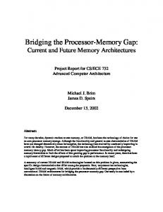
in [8]. The popularity of k-means is explainable by its low computational complexity and well understood mathematical properties. However, k-means will only find non-optimal local-minima, depending on the initial configuration of centroids. This is also known as the seeding problem and was addressed in various works. Recently a new strategy yielding better clustering results was introduced in [9]. Still, the runtime performance of k-means is a concern as data is growing rapidly, especially when finding the correct parameter of k can only be done by performing several runs with different numbers of clusters and initial seedings. With the appearance of programmable graphics hardware in 2001, using the GPU as a low-cost highly parallel streaming co-processor became a valuable option. Figure (I) illustrates the performance of GPUs and CPUs as well as differences in memory throughput over the years 2003 to 2008. This developement spawned scientific interest in this new architecture and resulted in numerous publications demonstrating the advantages of GPUs over CPUs when used for data parallel tasks. Much attention was focused on transferring common parallel processing primitives to the GPU and creating frameworks to allow for more general purpose programming [10, 11]. The most problematic aspect of this undertaking was transforming the problems at hand into a graphics processor pipeline friendly format, a task needing knowledge about graphics programming. The reader is referred to [12] where an in-depth discussion on mapping computational concepts to the GPU can be found. This entry barrier was recently lowered by the introduction of NVIDIA’s CUDA [13] as well as ATI’s Close to Metal Initiative [14]. Both were designed to enable direct exploitation of the hardware’s capabilities circumnavigating the invocation of the graphics pipeline via an API such as OpenGL or DirectX. In this work CUDA was chosen due to its more favorable properties, namely the high-level approach employed by its seamless integration with C and the quality of its documentation. In this paper a parallel implementation of k-means on the GPU via CUDA is discussed. Section II discusses the sequential and parallel variants of k-means leading to Section III where related work is investigated. Section IV gives an overview of CUDA’s properties and programming
International Journal on Advances in Systems and Measurements, vol 2 no 2&3, year 2009, http://www.iariajournals.org/systems_and_measurements/
225
Figure 2. clusters.
A simple two dimensional toy example with three gaussian
cluster centroids. The optimal set C of k centroids can be found by minimizing the following potential function: φ=
n X i=1
min D(xi , cj )2
cj ∈C
(1)
D is a metric in Rd , usually the euclidean distance. Solving Equation (1) even for two clusters was proven to be NP-hard in [16]. However, a non-optimal solution for the kmeans problem exists and will be described in the following subsection. For the rest of the discussion it is assumed that the set of data points X is already available in-core, that is loaded to memory. Figure 1. [15]
Evolution of CPU and GPU performance over the last decade
B. Sequential K-Means
model followed by Section V describing the concrete parallel implementation of k-means on the GPU. A comparison of the GPU implementation versus an optimized sequential CPU implementation is given in Section VI. Finally, Section VII concludes this paper. II. K-M EANS C LUSTERING In this section a definition of the k-means problem is given as well as non-optimal sequential and parallel algorithmic solutions. Additionally the computational complexity is discussed. A. Problem Definition The k-means problem can be defined as follows: a set X of n data points xi ∈ Rd , i = 1, . . . , n as well as the number of clusters k ∈ N+ < n is given. A cluster Cj ⊂ X , j = 1, . . . , k with a centroid cj ∈ Rd is composed of all points in X for which cj is the nearest centroid. The distance from a data point to a centroid is determined by some suitable metric. Figure (II-A) shows a simple toy dataset with 3 gaussian clusters, some outliers and the 3
In [8] MacQueen describes an algorithm that locally improves some clustering C by iteratively refining it. An initial clustering C is created by choosing k random centroids from the set of data points X . This is known as the seeding stage. Next a labeling stage is executed where each data point xi ∈ X is assigned to the cluster Cj for which D(xi , cj ) is minimal. Each centroid cj is then recalculated P by the mean of all data points xi ∈ Cj via cj = |C1j | xi ∈Cj xi . The labeling and centroid update stage are executed repeatedly until C no longer changes. This procedure is known to converge to a local minimum subject to the initial seeding [17]. Algorithm 1 describes the procedure in algorithmic terms. The next subsection demonstrates how this sequential algorithm can be transformed into a parallel implementation. C. Parallel K-Means In [18] Dhillon presents a parallel implementation of kmeans on distributed memory multiprocessors. The labeling stage is identified as being inherently data parallel. The set of data points X is split up equally among p processors, each calculating the labels of all data points of their subset
International Journal on Advances in Systems and Measurements, vol 2 no 2&3, year 2009, http://www.iariajournals.org/systems_and_measurements/
226 Algorithm 1 Sequential K-Means Algorithm cj ← random xi ∈ X , j = 1, . . . , k, s.t. cj 6= ci ∀i 6= j repeat Cj ← ∅, j = 1, . . . , k for all xi ∈ X do j ← arg minD(cj , xi ) Cj ← Cj ∪ xi end for for all cj ∈ P C do cj ← |C1j | xi ∈Cj xi end for until convergence
of X . In a reduction step the centroids are then updated accordingly. It has been shown that the relative speedup compared to a sequential implementation of k-means increases nearly linearly with the number of processors. Performance penalties introduced by communication cost between the processors in the reduction step can be neglected for large n. Algorithm 2 Parallel K-Means Algorithm if threadId = 0 then cj ← random xi ∈ X , j = 1, . . . , k, s.t. cj 6= ci ∀i 6= j end if synchronize threads repeat for all xi ∈ XthreadId do li ← arg minD(cj , xi ) end for synchronize threads if threadId=0 then for all xi ∈ X do cli ← cli + xi mli ← mli + 1 end for for all cj ∈ C do cj ← m1j cj end for if convergence then signal threads to terminate end if end if until convergence Since the GPU is a shared memory multiprocessor architecture this section briefly outlines a parallel implementation on such a machine. It only slightly diverges from the approach proposed by Dhillon. Processors are now called threads and a master-slave model is employed. Each thread is assigned an identifier between 0 and t−1 where t denotes the number of threads. Thread 0 is considered the master thread,
all other threads are slaves. Threads share some memory within which the set of data points X , the set of current centroids C as well as the clusters Cj reside. Each thread additionally owns local memory for miscellaneous data. It is further assumed that locking mechanisms for concurrent memory access are available. Given this setup the sequential algorithm can be mapped to this programming model as follows. The master thread initializes the centroids as it is done in the sequential version of k-means. Next X is partitioned into subsets Xi , i = 0, . . . t. This is merely an offset and range calculation each thread executes giving those xi each thread processes in the labeling stage. All threads execute the labeling stage for their partition of X. The label of each data point xi is stored in a component li of an n-dimensional vector. This eliminates concurrent writes when updating clusters and simplifies bookkeeping. After the labeling stage the threads are synchronized to ensure that all data for the centroid update stage is available. The centroid update stage could then be executed by a reduction operation. However, for the sake of simplicity it is assumed that the master thread executes this stage sequentially. Instead of iterating over all centroids the master thread iterates over all labels partially calculating the new centroids. A k-dimensional vector m is updated in each iteration where each component mj holds the number of data points assigned to cluster Cj . Next another loop over all centroids is performed scaling each centroid cj by m1j giving the final centroids. Convergence is also determined by the master thread by checking whether the last labeling stage introduced any changes in the clustering. Slave threads are signaled to stop execution by the master thread as soon as convergence is achieved. Algorithm 2 describes the procedure executed by each thread. D. Computational Complexity In this section the number of operations executed by kmeans in each iteration is investigated. This number is equal for both implementations. It therefore serves as the basis for comparing runtime behavior in section VI. For the computational complexity analysis each floating point operation is counted as one computational unit. Additions, multiplications and comparisons are considered to be floating point operations. Also, the seeding stage is ignored in this analysis. The labeling stage consists of evaluating the distance from each data point xi to each centroid cj . Given an euclidean distance metric each distance calculation consists of one subtraction, one multiplication and one addition per dimension totaling in 3d operations. Additionally a square root is calculated adding another operation per distance calculation. Finding the centroid nearest to a data point xi is an iterative process where in each iteration a comparison between the last minimal distance and the current distance is
International Journal on Advances in Systems and Measurements, vol 2 no 2&3, year 2009, http://www.iariajournals.org/systems_and_measurements/
227
performed. This adds another operation to the total number of operations per labeling step. There is a total of nk labeling steps resulting in the total numbers of operations of Olabeling = 3nkd + 2nk = nk(3d + 2)
(2)
for the labeling stage in each iteration. In each iteration of the centroid update stage the mean for each cluster Cj is calculated consisting of adding |Cj | ddimensional vectors as well as dividing each component of the resulting vector by |Cj |. In total n d-dimensional vectors are added yielding nd operations plus kd operations for the scaling of each centroid cj by |C1j | . For the update stage there are thus Oupdate = nd + kd = d(n + k)
(3)
operations executed per k-means iteration. The total number of operations per k-means iteration is given by Oiteration = Olabeling + Oupdate = nk(3d + 2) + d(n + k) (4) From Equations (2) and (3) it can be observed that the labeling stage is clearly the most costly stage per iteration. If d n and k n the updating stage contributes insignificantly to the total number of operations making the labeling stage the dominant factor. III. R ELATED W ORK To the best of the authors’ knowledge, three different implementations of k-means on the GPU exist. All three implementations are similar to the parallel k-means implementation outlined in section II-C formulated as a graphics programming problem. Tabel (I) gives an overview of the various approaches. In [19] Takizawa and Kobayashi try to overcome the limitations imposed by the maximum texture size by splitting the data set and distributing it to several systems each housing a GPU. A solution to this problem via a multipass mechanism was not considered. Also the limitation on the maximum number of dimensions was not tackled. It is also not stated whether the GPU implementation produces the same results as the CPU implementation in terms of precision. Hall and Hart propose two theoretical options for solving the problem of limited instance counts and dimensionality: multi-pass labeling and a different data layout within the texture [20]. None of the approaches have been implemented though. In addition to the naive k-means implementation the data is reordered to minimize the number of distance calculations by only calculating the metrics to the nearest centroids. This is achieved by finding those centroids by traversing a previously constructed kd-tree. The authors could not observe any problems caused by the non standard
compliant floating point arithmetic implementations on the GPU, stating that the exact same clusterings have been found. The approach of Cao et. al. in [21] differs in that the centroid indices are stored in an 8-bit stencil buffer instead of the frame buffer limiting the number of total centroids to 256. Limitations in dimensionality and instance counts due to maximum texture sizes are solved via a costly multi-pass approach. No statements concerning precision of the GPU version were made. Summarizing the presented previous work the following can be observed: • All implementations suffer from architectural constraints such as maximum texture size limiting the number of instances, dimensions and clusters. The limitations can only be overcome by employing more costly multi-pass approaches. • Not all publications state the exact conditions the implementations were tested under. A direct comparison is not strictly possible. However, the given numbers indicate congruent results yielding an average speedup of a factor between 3 and 4. • The GPU implementation’s performance increases as the problem at hand grows bigger in dimensionality as well as instance and centroid count. • Only one paper mentioned potential impact of the non standard-compliant floating point arithemtics implemented on GPU’s. No effects have been observed. Based on the previous work the main contributions of this paper are as follows: 1) A parallel implementation of standard k-means on NVIDIA’s G80 GPU generation using the nongraphics oriented programming model of CUDA. 2) Removal of the limitations inherent to classical graphics-based general purpose GPU programming approaches for k-means, namely the number of instances, dimensions and centroids enabling large scale clustering problems to be tackled on the GPU. 3) Investigation of precision issues due to the non IEEE single precision floating point compliance of modern GPU’s. 4) Performance evaluation of the presented implementation in comparison to an aggressively optimized single core CPU implementation, using SSE3 vectorization as well as loop unrolling optimizations, showing high speedups when compared to the average speedup of previous GPU-based implementations. 5) Evaluation of on-chip memory throughput as well as floating point operation performance. IV. CUDA With the advent of the unified shader model the separation of vertex and fragment shader processors in hardware
International Journal on Advances in Systems and Measurements, vol 2 no 2&3, year 2009, http://www.iariajournals.org/systems_and_measurements/
228
CPU Compiler Optimizations GPU Speedup
Takizawa and Kobayashi [19] Intel P4 3.2 Ghz GNU C++ 3.3.5 SSE2 NVIDIA Geforce 6600 Ultra 4
Hall and Hart [20] AMD Athlon 2800+ ? ? NVIDIA GeforceFX 5900 2-3
Cao et. al. [21] Intel P4 3.4 Ghz Intel C++ SSE2, Hyper-Threading NVIDIA Geforce 6800 GT 4
Table I S UMMARY OF PREVIOUS GPU- BASED K - MEANS IMPLEMENTATIONS . T HE COLUMN SPEEDUP GIVES THE RELATIVE SPEEDUP OF THE GPU VERSION TO THE CPU VERSION BASED ON TOTAL RUNTIME
has vanished. Shader processors can now be configured to perform both tasks depending on the requirements of the application [22]. Starting from the G80 family of GPUs NVIDIA supports this new shader model resulting in a departure from previous GPU designs. The GPU is now composed of so called multiprocessors that house a number of streaming processors ideally suited for massively dataparallel computations. NVIDIA’s CUDA is build on top of this new architecture eliminating the need to reformulate computations to the graphics pipeline. The GPU is viewed as a set of multiprocessors executing concurrent threads in parallel. Threads are grouped into thread blocks and execute the same instruction on different data in parallel. One or more thread blocks are directly mapped to a hardware multiprocessor where time sharing governs the execution order. Within one block threads can be synchronized at any execution point. A certain execution order of threads within a block is not guaranteed. Blocks are further grouped into a grid, communication and synchronization among blocks is not possible; execution order of blocks within a grid is undefined. Threads and blocks can be organized in three and two dimensions respectively. A thread is assigned an id depending on its position in the block. A block is also given an id depending on its position within a grid. Figure (IV shows a two dimensional grid of 2 by 3 thread blocks. Each thread block is composed of 3 by 4 threads. The thread and block id of a thread is accessible at runtime allowing for specific memory access patterns based on the chosen layouts. Each thread on the GPU executes the same procedure known as a kernel [15]. Threads have access to various kinds of memory. Each thread has very fast thread local registers and local memory assigned to it. Within one block all threads have access to block local shared memory that can be accessed as fast as registers depending on the access patterns. Registers, local memory and shared memory are limited resources. Portions of device memory can be used as texture or constant memory which benefit from on-chip caching. Constant memory is optimized for read-only operations, texture memory for specific access patterns. Threads also have access to uncached general purpose device memory or global memory [15]. Figure (IV) gives an overview of this architecture. Various pitfalls exist that can degrade performance of the GPU. Shared memory access by multiple threads in parallel
Figure 3. A grid of thread blocks. Each thread block is composed of a number of threads. Blocks and threads are indexed [15]
can produce so called bank conflicts serializing execution of those threads and therefore reducing parallelism. Second, when accessing global memory addresses have to be a multiple of 4, 8 or 16, otherwise an access might be compiled to multiple instructions and therefore accesses. Also, addresses accessed simultaneously by multiple threads in global memory should be arranged so that memory access can be coalesced into a single continuous aligned memory access. This is often referred to as memory coalescing. Another factor is so called occupancy. Occupancy defines how many blocks and therefore threads are actually running in parallel. As shared memory and registers are limited resources the GPU can only run a specific number of blocks in parallel. It is therefore mandatory to optimize the usage of shared memory and registers to allow to run as many blocks and threads in parallel as possible [15]. The CUDA SDK gives the developer easy to use tools that fully integrate with various C++ compilers. Code for the GPU is written in a subset of C with some extensions
International Journal on Advances in Systems and Measurements, vol 2 no 2&3, year 2009, http://www.iariajournals.org/systems_and_measurements/
229
/ / f e t c h t h e r e s u l t f r o m t h e gpu .. }
Figure 4. Hardware view of the CUDA architecture showing interdependancies and various forms of memory [15]
and can coexist with CPU (host) code in the same source file. The host code is responsible for setting up the layout of blocks and threads as well as uploading data to the GPU. Kernel execution is performed asynchronously, primitives to synchronize between CPU and GPU code are available. Debugging of device code is possible but only in an emulation environment that runs the kernel on the CPU in heavyweight threads which does not simulate all peculiarities of the GPU. Below a simple example for substracting two vectors is given: global
void sub ( f l o a t ∗ a , float∗ b , f l o a t ∗ out )
A CUDA program most often follows this sequence of steps. First the data on which the computations should be caried out is fetched from a source, e.g. a file on disk and loaded into RAM. Next the CUDA API is used to allocate memory on the GPU and the data is transfered to this newly allocated space. The API returns pointers that can be used as arguments for a kernel invocation later on. At kernel invocation time the number of thread blocks and blocks within a thread is specified and any arguments are passed in. In the above example each thread in the block will calculate the difference of one dimension of the two vectors and place the result in the corresponding element in array out. The index is derived from the threads id given by threadIdx.x. After the kernel has finished the result, for which memory on the GPU was also allocated previously, is transfered back to RAM. Of course this simple example leaves out a lot of features and capabilities offered by the API and special purpose language extensions. For an excellent introduction to CUDA the reader is refered to [23]. The integration with C is seamless, functions marked with the global modifier will be compiled by the NVIDIA nvcc compiler, yielding binary code executable by the GPU. Kernel invocations will also be replaced with code that loads the binary code to the GPU and invokes some driver functions to execute it. V. PARALLEL K-M EANS VIA CUDA This section describes the CUDA based implementation of the algorithm outlined in section II-C. In the first sub section the overall program flow is described. The next subsection presents the labeling stage on the GPU followed by section V-C outlining the data layout used and CUDA specific optimizations employed to further speed up the implementation. A. Program Flow
{ int i = threadIdx . x ; out [ i ] = a [ i ] − b [ i ] ; } i n t main ( ) { / / i n i t i a l i z e cuda ... / / a l l o c a t e and f i l l memory ... / / execute the kernel sub (a , b , c ) ;
The CPU takes the role of the master thread as described in section II-C. As a first step it prepares the data points and uploads them to the GPU. As the data points do not change over the course of the algorithm they are only transfered once. The CPU then enters the iterative process of labeling the data points as well as updating the centroids. Each iteration starts by uploading the current centroids to the GPU. Next the GPU performs the labeling as described in section V-B. The results from the labeling stage, namely the membership of each data point to a cluster in form of an index, are transfered back to the CPU. Finally the CPU calculates the new centroid of each cluster based on these labels and performs a convergence check. Convergence is achieved in case no label has changed compared to the last iteration. Optionally a thresholded difference check of the
International Journal on Advances in Systems and Measurements, vol 2 no 2&3, year 2009, http://www.iariajournals.org/systems_and_measurements/
230
overall movement of the centroids can be performed to avoid iterating infinitely for some special cluster configurations. B. Labeling Stage The goal of the labeling stage is to calculate the nearest centroid for each data point and store the index of this centroid for further processing by the centroid update stage on the CPU. Therefore each thread has to calculate which data points it should process, label it with the index of the closest centroid and repeat this for any of its remaining data points. The task for each thread is thus divided into two parts: calculate and iterate over all data points belong to the thread according to a partitioning schema and performing the actual labeling for the current data point. The following paragraphs will thus first discuss the partitioning schema and the first part of this task followed by a description of the actual labeling step. As discussed in section IV the GPU slightly differs from the architecture assumed in section II-C. Threads are additionally grouped into blocks that share local memory. Instead of assigning each thread a chunk of data points, each block of threads is responsible for one or more chunks. One such chunk contains t data points where t is the number of threads per block. As the amount of threads per block as well as blocks is limited by various factors, such as used registers, each block processes not only one but several chunks depending on the total amount of data points. Denoting the amount of data points by n then nchunks = dn/te
(5)
gives the number of chunks to be processed. Note that the last chunk does not have to be fully filled as n does not have to be a multiple of t. This chunks have to be partitioned among the number of blocks b. Two situations can arise: 1) nchunks mod b = 0, no block is idle 2) nchunks mod b 6= 0, b − nchunks blocks are idle Therefore each block processes at least bnchunks /bc chunks. The first nchunks mod b blocks process the remaining chunks. For each chunk one thread within a block labels exactly one data point. For chunks that have less data points than there are threads within a block some threads will be idle and not process a data point. Based on the partitioning schema described each thread processes at most nchunks data points. For each data point a thread therefore has to calculate the index of the data point based on it’s block and thread id. This is done iteratively in a loop. The thread starts by calculating the index of its data point of the first chunk to be processed by the thread’s block expressed by block.id + thread.id. In each iteration the next data point’s index is calculating by adding tb to the last data points index. In case the calculated index is bigger than n − 1 the thread has processed all it’s data points. No thread can terminate before the other threads within the same block so any thread
that is done processing all its data points has to wait for the other threads to finish processing their remaining data points. Therefore each thread iterates dn/tbe times and simply does not execute the labeling code in case its current data point index is bigger than n−1. To minimize the number of idling threads it is therefore mandatory to adjust the number of blocks to the number of data points minimizing n mod tb. The actual labeling stage is again composed of two distinct parts. A thread has to calculate the distance of its current data point to each centroid. In the implementation presented here all threads within a block calculate the distance to the same centroid at any one time. This allows loading the current centroid to the block’s local shared memory accessible by all threads within the block. For each centroid the threads within the block therefore each load a component of the current centroid to shared memory. Each thread then calculates the distance from their data point to the centroid in shared memory fetching the data point’s components from global memory in a coalesced manner. See section V-C on the data layout used for coalescing reads and writes. Loading the complete centroid to memory limits the amount of dimensions as shared memory is restricted to some value, on the hardware used it’s 16 kilobytes. Given that components are encoded as 32-bit floating point values this roughly equals a maximum dimension count of 4000. To allow for unlimited dimensions the process of loading and calculating the distance from a data point to a centroid is done in portions. In each iteration t components of the centroid are loaded to shared memory. For each component the partial euclidean distance is calculated. Depending on d not all threads have to take part in loading the current components to memory, so some threads might idle. When all threads have evaluated the nearest centroid the resulting label, being the index of the centroid a data point is nearest to, is written back to global memory. The labels for each data point are stored in an additional vector component. After all blocks have finished processing their chunks the CPU is taking over control again, downloading the labels calculated for constructing the new centroids and checking for convergence. The next section describes the data layout as well as other optimizations. C. Data Layouts & Optimizations A GPU-based implementation of an algorithm that is memory bound, as is the case with k-means, can yield very poor performance when the GPU’s specifics are not taken into account. For memory throughput these specifics depend on the memory type used for storing and accessing data on the GPU as described in section IV. For the k-means implementation presented in this paper global memory was chosen as the storage area for the data points and centroids. As data points are only read during the labeling stage on the GPU, storage in constant or texture memory might have increased memory throughput to some degree. However,
International Journal on Advances in Systems and Measurements, vol 2 no 2&3, year 2009, http://www.iariajournals.org/systems_and_measurements/
231
texture and constant memory restrict the maximum amount of data and therefore processable data points and centroids, a drawback earlier GPU-based k-means implementations suffered from as described in section III. Global memory on the other hand allows gather and scatter operations and permits to use almost all of the memory available on the GPU. For global memory coalescing reads and writes are mandatory to achieve the best memory throughput. All vectors are assumed to be of dimensionality d and stored in dense form. As described in the last section centroids are loaded from global memory to shared memory in portions, each portion being made up of at most t components. As t threads read in subsequent components at once the centroids are stored as rows in a matrix, achieving memory coalescing. Data points are stored differently due to the order in which components are accessed. Here, each thread accesses one component of its current data point simultaneously to the other threads. Therefore data points are stored column wise again providing memory coalescing. Additionally a component is added as the first component of each vector where each threads writes the label of the closes centroid to for further processing by the CPU. This layout also allows downloading this labels in a bulk operation. For both centroids and data points special CUDA API methods where used that allocate memory at address being a multiple of 4 yielding the best performance. As the implementation of k-means using an euclidean distance metric is clearly memory bound further optimizations have been made by increasing occupancy. This was achieved by decreasing the amount of registers each thread uses. Specifically counter variables for the outer loops are stored in shared memory. This optimization increased performance by around 25%. The program executed by each thread uses 10 registers. The optimal number of threads is therefore 128 according to the NVIDIA CUDA Occupancy Calculator included in the CUDA SDK. As descibed in section V-B partial or entire thread blocks can be idle depending on the ratio between the number of blocks and threads within a block to the number of data points. To reduce the effect of idle blocks on performance the block count is adapted to the number of data points to be processed, minimizing nchunks mod b. The next section discusses experiments and their results for the k-means implementation presented in this section. VI. E XPERIMENTS & R ESULTS Experimental results were obtained on artificial data sets. As the performance is not dependent on the actual data distribution the synthetic data sets were composed of randomly placed data points. To observe the influence of the number of data points on the performance data sets with 500, 5000, 50,000 and 500,000 instances were created. For
each instance count 3 data sets were created with 2, 20 and 200 dimensions. The sequential k-means implementation and the centroid update phase for the gpu-base k-means was coded in C using the Visual C++ 2005 compiler as well as the Intel C++ compiler 10.1. For both compilers full optimizations were enabled, favoring speed over size as well as using processor specific extensions like SSE3. In the case of the Intel C++ compiler all vector related operations such as distance measurements, additions and scaling were vectorized using SSE3. The CUDA portions of the code were compiled using the CUDA Toolkit 2.0. We evaluated our implementation on two systems. The first one which we will refer to as System 1 was composed of an Intel Core 2 Duo E8400 CPU, 4 GB RAM running Windows XP Professional with Service Pack 3. The GPU was an NVIDIA GeForce 9600 GT hosting 512 MB of RAM, the driver used was the NVIDIA driver for Windows XP with CUDA support version 178.08. The second system, refered to as System 2 was made of an Intel Core 2 Quad Q9550, 4 GB RAM running Windows 7 RC build 7100 and the NVIDIA driver for Windows 7 with CUDA support version 190.39. We first discuss the findings on System 1 and then briefly analyse the results from System 2. Figures 5 and 6 present the speedups gained by using the GPU relative to the CPU implementation on System 1. While full optimizations were turned on for the Visual C++ version the GPU-based implementation outperformed it by a factor of 4 to 43 for all but the smallest data set. A clear increase in performance can be observed the higher the number of instances dimensions and clusters. Due to the poor results of Visual C++ we omit further measurements and concentrate on the results produced by the Intel C++ version. For the fully optimized Intel C++ version the speedups are obviously smaller as this version makes use of the SIMD instruction-set of the CPU. A speedup by a factor of 1.5 to 14 can be observed for all but the smallest data set on System 1. Interestingly this version performs better for lower dimensionality for high instance counts. This is due to the fact that as the centroid update time decreases due to optimization the transfer time starts to play a bigger role. Nevertheless there is still a considerable speedup observable. The diagrams in figure 7 also explain why the GPU-based implementation does not match the CPU implementation for very small data sets. From the plot it can be seen that for 500 data points nearly all the time is spent on the GPU. This time span also includes the calling overhead for invoking the GPU labeling stage. This invocation time actually takes longer than labeling the data items. The GPU-based implementation is clearly memory bound as there are more memory accesses than floating point operations. Figure 8 shows the throughput achieved by the GPU for various dataset sizes. A peak throughput of 44GB/s could be achieved for the largest problem with 500000 instances
International Journal on Advances in Systems and Measurements, vol 2 no 2&3, year 2009, http://www.iariajournals.org/systems_and_measurements/
232 500 Points
5000 Points
2,5
25
2
20
500 Points
5000 Points 4,5
0,5 0,45
4
0,4
200 1
0,5
2
0,35
20 200 10
5
3
0,3
Speedup
20
2 20
0,25
200
0,2
Speedup
15
2
Speedup
Speedup
1,5
3,5
0
Clusters
32
64
128
2
4
8
16
Clusters
32
64
0,5
0,05
128
0
0 2
45
35
40
200
15
25
10
4
8
16
32
Clusters
64
128
5
5
0
0 64
128
500.000 Points 14
12
10 6
200
10
32
2
128
7
20
20 15
16
64
8
2
Speedup
20
20
Speedup
Speedup
2
Clusters
32
50.000 Points
30 25
8
16
Clusters
9
35
30
4
8
500.000 Points
50.000 Points 40
2
4
2
5
20 200
4
2
8
Speedup
16
20 200
6
3 4 2 2
4
8
16
Clusters
32
64
2
1
128
0
0 2
16
Clusters
32
64
128
2
500 Points, 200 Dimensions
4
8
16
Clusters
32
64
128
500.000 Points, 200 Dimensions
100%
100%
90%
90%
80%
80%
70%
70% Transfer
60%
Time
with 200 dimensions and 128 clusters. For the used hardware the peak performance is given as 57.6 GB/s. Therefore we are highly confident that the implementation is nearly optimal. For very small datasets the throughput is not even one percent of the reachable peak performance. Interestingly, for the dataset with 500 instances, 200 dimensions and 128 clusters a sharp deviation from an otherwise log like curve can be observed. This indicates a sweetspot at which the graphics card is able to benefit from the data size. Due to being memory bound the GFLOP counts do of course not reach the hardwares peak values. Figure 9 shows the approximate GFLOP/s achieved by our implementation. As with memory transfers the performance gets better the more data is thrown at the hardware. Also, the spike in the small dataset that was found in the memory throughput analysis can also be found here for the same reason as stated above: given a certain dataset size the graphics card is better able to benefit from its inherent parallel nature. We repeated the measurements for System 2. Figures 10 through 13 present the results from System 2. The relative performance compared to the CPU version does not increase immensely. However, one has to take into account the the CPU used on System 2 is also better than the one used for relative measurements on System 1. The trend is very similar to the one observed on System 1. We achieve near peak memory throughput but can not exploit the computational capabilities fully. Additionally the performance decreases a
8
Figure 6. Speedup measured against Intel C++ compiler for various instance counts and dimensions on System 1
Labeling
50% 40%
Transfer
60%
Centroid Update
Centroid Update Labeling
50% 40%
30%
30%
20%
20%
10%
10%
0%
0% 2
4
8
16
Clusters
32
64
128
2
50.000 Points, 200 Dimensions
4
8
16
Clusters
32
64
128
5000 Points, 200 Dimensions
100%
100%
90%
90%
80%
80%
70%
70% Transfer
60%
Time
Figure 5. Speedup measured against the Visual C++ compiler for various instance counts and dimensions on System 1
4
Time
8
Labeling
50% 40%
Centroid Update Labeling
50% 40%
30%
30%
20%
20%
10%
10%
0%
Transfer
60%
Centroid Update
Time
4
200
1
0,1 2
20
2 1,5
0,15
0
2
2,5
0% 2
4
8
16
Clusters
32
64
128
2
4
8
16
Clusters
32
64
128
Figure 7. Percentage of time used for the different stages on the GPU on System 1
International Journal on Advances in Systems and Measurements, vol 2 no 2&3, year 2009, http://www.iariajournals.org/systems_and_measurements/
233 500 Points 500 Points
5000 Points
6,0
25,0
5,0
5000 Points
0,35
3,5
0,3
3
0,25
2,5
20,0 2
2
20
3,0
20 200
GB/S
GB/S
200
200
20 200
0,1
1
0,05
0,5
5,0
0
0 2
0,0
2
2
1,5
10,0
2,0
1,0
20
0,15
Speedup
15,0
2
Speedup
0,2 4,0
4
8
16
Clusters
32
64
128
2
4
2
4
8
16
Clusters
32
64
128
2
4
8
16
Clusters
32
64
500.000 Points
32
64
128
35,0
50,0
9
45,0
8
40,0
7
30,0
20
20,0
20
25,0
GB/s
200
15,0
2 200
16
Clusters
32
64
128
2
4
8
16
Clusters
32
64
500 Points
5000 Points 16,0
4,0
14,0
3,5
12,0
3,0 10,0
2,5
20 200
2,0
GFLop/S
2
1,5
2 20
8,0
200
6,0 4,0
1,0
2,0
0,5 0,0
0,0 2
4
8
16
Clusters
32
64
128
2
4
50.000 Points
8
16
Clusters
32
64
128
500.000 Points
30,0
35,0
30,0
25,0
2 20 200
10
5
0 4
8
16
Clusters
32
64
128
2
4
8
16
Clusters
32
64
128
128
Figure 8. Memory throughput for various instance counts and dimensions in Gigabytes on System 1
4,5
4
2
0,0 8
200
0
5,0
4
20
1
10,0
2
15
2
5
2
10,0
0,0
20
3
20,0 15,0
5,0
Speedup
30,0
2
25
6
35,0 25,0
500.000 Points
10
Speedup
40,0
GB/S
16
Clusters
128
50.000 Points 50.000 Points
GFlop/S
8
0,0
Figure 10. Speedup measured against Intel C++ compiler for various instance counts and dimensions on System 2
little as the number of clusters and dimensions increases for the largest dataset. We do not have an explanation for this behaviour and will investigate this in future work. However, from the timing chart it is clear the the GPU is doing a lot less work in total compared to the work it did in System 1. Transfertimes play a much bigger role overall and the centroid update stage also takes up a bigger amount of time. It seems therefore advisable to keep the GPU saturated with more data in order to increase its overall contribution to performance. For some test runs slight variations in the resulting centroids were observed. These variations are due to the use of combined multiplication and addition operations (MADD) that introduce rounding errors. Quantifying these errors was out of the scope of this work, especially as no information from the vendor on the matter was available.
25,0 20,0
200
2
20,0
20
15,0
GFlop/s
GFlop/S
2
20 200
15,0
10,0 10,0 5,0
5,0
0,0
0,0 2
4
8
16
Clusters
32
64
128
2
4
8
16
Clusters
32
64
128
Figure 9. GFLOP/s reached for various instance counts and dimensions on System 1
VII. C ONCLUSION & F UTURE W ORK Exploiting the GPU for the labeling stage of k-means proved to be beneficial especially for large data sets and high cluster counts. The presented implementation is only limited in the available memory on the GPU and therefore scales well. However, some drawbacks are still present. Many real-life data sets like document collections operate in very high dimensional spaces where document vectors are sparse. The implementation of linear algebra operations on sparse data on the GPU has yet to be solved optimally. Necessary access patterns such as memory coalescing make
International Journal on Advances in Systems and Measurements, vol 2 no 2&3, year 2009, http://www.iariajournals.org/systems_and_measurements/
234 500 Points 500 Points, 200 Dimensions
5000 Points, 200 Dimensions
90%
6,0
80%
80%
5,0
70%
70% Transfer Centroid Update Labeling
50% 40%
Transfer
60%
Centroid Update Labeling
50%
1,0
20%
0,0
10%
10%
0%
0% 8
16
32
64
200
2 20
15,0
200
10,0
2,0
40%
20%
Clusters
20
3,0
30%
4
20,0 2
4,0
30%
2
25,0
GFlop/s
90%
GFlop/s
100%
Time
Time
7,0
100%
60%
5000 Points 30,0
8,0
5,0
0,0 2
128
2
4
8
16
Clusters
32
64
4
8
16
Clusters
32
64
2
128
4
8
500.000 Points, 200 Dimensions 100%
90%
90%
80%
80%
70,0 100,0 60,0 80,0
60%
Centroid Update
Time
Labeling
50% 40%
Transfer Centroid Update Labeling
50%
GFlop/s
60%
Time
2
70% Transfer
40% 30%
20%
20%
200
30,0
10%
10%
0%
0% 8
16
32
Clusters
64
4
8
16
Clusters
32
64
500 Points
5000 Points
10,0 40,0 35,0 30,0 2
25,0
20
5,0
200
GFlop/s
GFlop/s
6,0
4,0 3,0 2,0
2 20
20,0
200
15,0 10,0
1,0
5,0
0,0 2
4
8
16
Clusters
32
64
0,0
128
2
4
8
16
Clusters
32
64
90,0
120,0
80,0 100,0
70,0 2 200
40,0 30,0
2
80,0
20
50,0
GFlop/s
GFlop/s
60,0
20 200
60,0
40,0
20,0 20,0 10,0 0,0
0,0 2
4
8
16
Clusters
32
64
128
2
4
8
16
Clusters
32
16
Clusters
32
64
128
2
4
8
16
Clusters
32
64
128
Figure 13. GFLOP/s reached for various instance counts and dimensions on System 1
this a very hard undertaking. Also, the implementation presented is memory bound meaning that not all of the GPUs computational power is harvested. Finally, due to rounding errors the results might not equal the results obtained by a pure CPU implementation. However, our experimental experience showed that the error is negligible. Future work will involve experimenting with other kmeans variations such as spherical or kernel k-means that promise to increase the computational load and therefore better suit the GPU paradigm. Also, an efficient implementation of the centroid update stage on the GPU will be investigated. R EFERENCES
140,0
100,0
8
128
500.000 Points
50.000 Points
4
128
Figure 11. Percentage of time used for the different stages on the GPU on System 1
7,0
0,0 2
2
8,0
200
20,0
10,0
128
9,0
20
60,0
20,0
0,0
4
2
20
40,0
40,0
30%
2
128
120,0
50,0 70%
64
500.000 Points
80,0
GFlop/s
100%
32
128
50.000 Points 50.000 Points, 200 Dimensions
16
Clusters
64
128
Figure 12. Memory throughput for various instance counts and dimensions in Gigabytes on System 1
[1] Mario Zechner and Michael Granitzer. Accelerating kmeans on the graphics processor via cuda. Intensive Applications and Services, International Conference on, 0:7–15, 2009. [2] A. K. Jain, M. N. Murty, and P. J. Flynn. Data clustering: a review. ACM Comput. Surv., 31(3):264– 323, September 1999. [3] Jian Yi, Yuxin Peng, and Jianguo Xiao. Color-based clustering for text detection and extraction in image. In MULTIMEDIA ’07: Proceedings of the 15th international conference on Multimedia, pages 847–850, New York, NY, USA, 2007. ACM. [4] Dannie Durand and David Sankoff. Tests for gene clustering. In RECOMB ’02: Proceedings of the sixth
International Journal on Advances in Systems and Measurements, vol 2 no 2&3, year 2009, http://www.iariajournals.org/systems_and_measurements/
235
[5]
[6] [7]
[8]
[9]
[10]
[11]
[12]
[13] [14]
[15]
[16]
[17]
annual international conference on Computational biology, pages 144–154, New York, NY, USA, 2002. ACM. Adil M. Bagirov and Karim Mardaneh. Modified global k-means algorithm for clustering in gene expression data sets. In WISB ’06: Proceedings of the 2006 workshop on Intelligent systems for bioinformatics, pages 23–28, Darlinghurst, Australia, Australia, 2006. Australian Computer Society, Inc. Shi Zhong. Efficient streaming text clustering. Neural Netw., 18(5-6):790–798, 2005. Stuart P. Lloyd. Least squares quantization in pcm. IEEE Transactions on Information Theory, 28(2):129– 136, 1982. J. B. MacQueen. Some methods for classification and analysis of multivariate observations. In L. M. Le Cam and J. Neyman, editors, Proc. of the fifth Berkeley Symposium on Mathematical Statistics and Probability, volume 1, pages 281–297. University of California Press, 1967. David Arthur and Sergei Vassilvitskii. k-means++: the advantages of careful seeding. In Nikhil Bansal, Kirk Pruhs, and Clifford Stein, editors, SODA, pages 1027– 1035. SIAM, 2007. Jens Kr¨uger and R¨udiger Westermann. Linear algebra operators for gpu implementation of numerical algorithms. In SIGGRAPH ’03: ACM SIGGRAPH 2003 Papers, pages 908–916, New York, NY, USA, 2003. ACM. Ian Buck, Tim Foley, Daniel Horn, Jeremy Sugerman, Kayvon Fatahalian, Mike Houston, and Pat Hanrahan. Brook for gpus: stream computing on graphics hardware. In SIGGRAPH ’04: ACM SIGGRAPH 2004 Papers, pages 777–786, New York, NY, USA, 2004. ACM. Mark Harris. Mapping computational concepts to gpus. In SIGGRAPH ’05: ACM SIGGRAPH 2005 Courses, page 50, New York, NY, USA, 2005. ACM. Nvidia cuda site, 2007. http://www.nvidia.com/object/ cuda home.html. Ati close to metal guide, 2007. http: //ati.amd.com/companyinfo/researcher/documents/ ATI CTM Guide.pdf. NVIDIA. NVIDIA CUDA Programming Guide 2.0. 2008. http://developer.download.nvidia.com/compute/ cuda/2 0/docs/NVIDIA CUDA Programming Guide 2.0.pdf. P. Drineas, A. Frieze, R. Kannan, S. Vempala, and V. Vinay. Clustering large graphs via the singular value decomposition. Mach. Learn., 56(1-3):9–33. Leon Bottou and Yoshua Bengio. Convergence properties of the K-means algorithms. In G. Tesauro, D. Touretzky, and T. Leen, editors, Advances in Neural Information Processing Systems, volume 7, pages 585–
592. The MIT Press, 1995. [18] Inderjit S. Dhillon and Dharmendra S. Modha. A dataclustering algorithm on distributed memory multiprocessors. In Large-Scale Parallel Data Mining, Lecture Notes in Artificial Intelligence, pages 245–260, 2000. [19] Hiroyuki Takizawa and Hiroaki Kobayashi. Hierarchical parallel processing of large scale data clustering on a pc cluster with gpu co-processing. J. Supercomput., 36(3):219–234, 2006. [20] Jesse D. Hall and John C. Hart. Gpu acceleration of iterative clustering. Manuscript accompanying poster at GP2: The ACM Workshop on General Purpose Computing on Graphics Processors, and SIGGRAPH 2004 poster (2004). [21] Feng Cao, Anthony K. H. Tung, and Aoying Zhou. Scalable clustering using graphics processors. In WAIM, pages 372–384, 2006. [22] David Luebke and Greg Humphreys. How gpus work. Computer, 40(2):96–100, 2007. [23] John Nickolls, Ian Buck, Michael Garland, and Kevin Skadron. Scalable parallel programming with cuda. In SIGGRAPH ’08: ACM SIGGRAPH 2008 classes, pages 1–14, New York, NY, USA, 2008. ACM.