k2 -trees for Compact Web Graph Representation? Nieves R. Brisaboa1 , Susana Ladra1 , and Gonzalo Navarro2 1
2
Database Lab., Univ. of A Coru˜ na, Spain. {brisaboa,sladra}@udc.es Dept. of Computer Science, Univ. of Chile, Chile.
[email protected] Abstract. This paper presents a Web graph representation based on a compact tree structure that takes advantage of large empty areas of the adjacency matrix of the graph. Our results show that our method is competitive with the best alternatives in the literature, offering a very good compression ratio (3.3–5.3 bits per link) while permitting fast navigation on the graph to obtain direct as well as reverse neighbors (2–15 microseconds per neighbor delivered). Moreover, it allows for extended functionality not usually considered in compressed graph representations.
1
Introduction
The World Wide Web structure can be regarded as a directed graph at several levels, the finest grained one being pages that point to pages. Many algorithms of interest to obtain information from the Web structure are essentially basic algorithms applied over the Web graph [16, 11]. Running typical algorithms on those huge Web graphs is always a problem. Even the simplest external memory graph algorithms, such as graph traversals, are usually non disk-friendly [24]. This has pushed several authors to consider compressed graph representations, which aim to offer memory-efficient graph representations that still allow fast navigation without decompressing. The aim of this research is to allow classical graph algorithms to be run in main memory over much larger graphs than those affordable with a plain representation. The most famous representative of this trend is surely Boldi and Vigna’s WebGraph Framework [6]. The WebGraph compression method is indeed the most successful member of a family of approaches to compress Web graphs based on their statistical properties [5, 7, 1, 23, 21, 20]. It allows fast extraction of the neighbors of a page while spending just a few bits per link (about 2 to 6, depending on the desired navigation performance). Their representation explicitly exploits Web graph properties such as: (1) the power-law distribution of indegrees and outdegrees, (2) the locality of reference, (3) the “copy property” (the set of neighbors of a page is usually very similar to that of some other page). More recently, Claude and Navarro [10] showed that most of those properties are elegantly captured by applying Re-Pair compression [17] on the adjacency lists, and that reverse navigation (finding the pages that point to a given page) ?
Funded in part (for the Spanish group) by MEC grant (TIN2006-15071-C03-03); and for the third author by Fondecyt Grant 1-080019, Chile.
2
Nieves R. Brisaboa, Susana Ladra, and Gonzalo Navarro
could be achieved by representing the output of Re-Pair using some more sophisticated data structures [9]. Reverse navigation is useful to compute several relevance ranking on pages, such as HITS, PageRank, and others. Their technique offers better space/time tradeoffs than WebGraph, that is, they offer faster navigation than WebGraph when both structures use the same space. Asano et al. [2] achieve even less than 2 bits per link by explicitly exploiting regularity properties of the adjacency matrix of the Web graphs, but their navigation time is substantially higher, as they need to uncompress full domains in order to find the neighbors of a single page. In this paper we also aim at exploiting the properties of the adjacency matrix, yet with a general technique to take advantage of clustering rather than a technique tailored to particular Web graphs. We introduce a compact tree representation of the matrix that not only is very efficient to represent large empty areas of the matrix, but at the same time allows efficient forward and backward navigation of the graph. An elegant feature of our solution is that it is symmetric, both navigations are carried out by similar means and achieve similar times. In addition, our proposal allows some interesting operations that are not usually present in alternative structures.
2
Our proposal
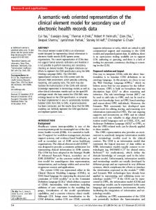
The adjacency matrix of a Web graph of n pages is a square matrix {aij } of n×n, where each row and each column represents a Web page. Cell aij is 1 if there is a hyperlink in page i towards page j, and 0 otherwise. Page identifiers are integers, which correspond to their position in an array of alphabetically sorted URLs. This puts together the pages of the same domains, and thus locality of reference translates into closeness of page identifiers. As on average there are about 15 links per Web page, this matrix is extremely sparse. Due to locality of reference, many 1s are placed around the main diagonal (that is, page i has many pointers to pages nearby i). Due to the copy property, similar rows are common in the matrix. Finally, due to skewness of distribution, some rows and colums have many 1s, but most have very few. We propose a compact representation of the adjacency matrix that exploits its sparseness and clustering properties. The representation is designed to compress large matrix areas with all 0s into very few bits. We represent the adjacency matrix by a k 2 -ary tree, which we call k 2 -tree, of height h = dlogk ne. Each node contains a single bit of data: 1 for the internal nodes and 0 for the leaves, except for the last level, where all are leaves and represent bit values of the matrix. The first level (numbered 0) corresponds to the root; its k 2 children are represented at level 1. Each child is a node and therefore it has a value 0 or 1. All internal nodes (i.e., with value 1) have exactly k 2 children, whereas leaves (with value 0 or at the last tree level) have no children. Assume for simplicity that n is a power of k; we will soon remove this assumption. Conceptually, we start dividing the adjacency matrix following a MXQuadtree strategy [22, Section 1.4.2.1] into k 2 submatrices of the same size, that is, k rows and k columns of submatrices of size n2 /k 2 . Each of the resulting k 2
k2 -trees for Compact Web Graph Representation
1
1
0
0
0
1
0
0
0
0
1
1 0
0
0
1
Retrieving direct neighbors for page 10
page 10
1 1101
0
0
3
1 11 10
(a) First example.
0
1
0
0
0
0
0
0
0
0
0
0
0
0
0
0
0
0
1
1
1
0
0
0
0
0
0
0
0
0
0
0
0
0
0
0
0
0
0
0
0
0
0
0
0
0
0
0
0
0
0
0
0
0
0
0
0
0
0
0
0
0
0
0
0
0
0
0
0
0
0
0
0
0
0
0
0
0
0
0
0
0
0
0
0
0
0
0
0
0
0
0
0
0
0
0
0
0
0
0
0
0
0
0
0
0
0
0
0
0
0
0
0
0
0
0
0
0
1
0
0
0
0
0
0
0
0
0
0
0
0
0
0
0
1
0
0
0 1
0
0
0
0
0
0
0
0
0
0
0
0
1
0
0 1
0
0 1
0
0
0
0
0
0
0
0
0
0
0
1
0
0
0 1
0
0
0
0
0
0
0
0
0
0
0
0
0
0
0
0
0
0
0
0
0
0
0
0
0
0
0
0
0
0
0
0
0
0
0
0
0
0
0
0
0
0
0
0
0
0
0
0
0
0
0
0
0
0
0
0
0
0
0
0
0
0
0
0
0
0
0
0
0
0
0
0
0
0
0
0
0
0
0
0
0
0
0
0
0
0
1
1 1
100
0100 0011
0
1 1 0 00 0010
0
1
0
1 0 0 01 0010
1
01 0 1 1010 1000
1
0
0 1
1 1
0
0
0
1 0
0110 0010 0100
(b) Expansion, subdivision and navigation for k = 2. Fig. 1. k2 -tree examples.
submatrices will be a child of the root node and its value will be 1 iff in the cells of the submatrix there is at least one 1. A 0 child means that the submatrix has all 0s and hence the tree decomposition ends there. The children of a node are ordered in the tree starting with the submatrices in the first (top) row, from left to right, then the submatrices in the second row from left to right, and so on. Once the level 1, with the children of the root, has been built, the method proceeds recursively for each child with value 1, until we reach submatrices full of 0s, or we reach the cells of the original adjacency matrix. In the last level of the tree, the bits of the nodes correspond to the matrix cell values. Figure 1(a) illustrates a 22 -tree for a 4 × 4 matrix. A larger k induces a shorter tree, with fewer levels, but more children per internal node. If n is not a power of k, we conceptually extend our matrix to the right and bottom with 0s, making it of width n0 = k dlogk ne . This does not cause a significant overhead as our technique is efficient to handle large areas of 0s. Figure 1(b) shows an example of the adjacency matrix of a Web graph (we use the first 11 × 11 submatrix of graph CNR [6]), how it is expanded to an n0 × n0 matrix (n0 power of k = 2) and its corresponding tree. Notice that its last level represents cells in the original adjacency matrix, but most cells in the original adjacency matrix are not represented in this level because, where a large area with 0s is found, it is represented by a single 0 in a smaller level of the tree. 2.1
Navigating with a k2 -tree
To obtain the pages pointed by a specific page p, that is, to find direct neighbors of page p, we need to find the 1s in row p of the matrix. We start at the root and travel down the tree, choosing exactly k children of each node. Example. We find the pages pointed by the first page in the example of Figure 1(a), that is, find the 1s of the first matrix row. We start at the root of the 22 -tree and compute which children of the root overlap the first row of the matrix. These are the first two children, to which we move: – The first child is a 1, thus it has children. To figure out which of its children are useful we repeat the same procedure. We compute in the corresponding submatrix (the one at the top left corner) which of its children represent cells overlapping the first row of the original matrix. These are the first and the second children. They are leaf nodes and their values are 1 and 1.
4
Nieves R. Brisaboa, Susana Ladra, and Gonzalo Navarro
– The second child of the root represents the second submatrix, but its value is 0. This means that all the cells in the adjacency matrix in this area are 0. Thus, the Web page represented by the first row has links to itself and page 2. Figure 1(b) shows this navigation for a larger example. Reverse neighbors. An analogous procedure retrieves the list of reverse neighbors. To obtain which pages point to page q, we need to locate which cells have a 1 in column q of the matrix. Thus, we carry out a symmetric algorithm, using columns instead of rows. Summarizing, searching for direct or for reverse neighbors in the k 2 -tree is completely symmetric. The only difference is the formula to compute the children of each node used in the next step. In either case we perform a top-down traversal of the tree. If we want to search for direct(reverse) neighbors in a k 2 -tree, we go down through k children forming a row(column) inside the matrix.
3
Data structure and algorithms
Our data structure is essentially a compact tree of N nodes. There exist several such representations for general trees [14, 19, 4, 12], which asymptotically approach the information-theoretic minimum of 2N + o(N ) bits. In our case, where there are only arities k 2 and 0, the information-theoretic minimum of N + o(N ) bits is achieved by a so-called “ultra-succinct” representation [15] for general trees. Our representation is much simpler, and close to the so-called LOUDS (level-ordered unary degree sequence) tree representation [14] (which would not achieve N + o(N ) bits if directly applied to our trees). Our data structure can be regarded as a simplified variant of LOUDS for the case where arities are just k 2 and 0, which achieves the information-theoretic minimum of N +o(N ) bits, provides the traversal operations we require (basically move to the i-th child, although also parent is easily supported) in constant time, and is simple and practical. 3.1
Data structure
We represent the whole adjacency matrix via the k 2 -tree using two bit arrays: T (tree): stores all the bits of the k 2 -tree except those in the last level. The bits are placed following a levelwise traversal: first the k 2 binary values of the children of the root node, then the values of the second level, and so on. L (leaves): stores the last level of the tree. Thus it represents the value of (some) original cells of the adjacency matrix. We create over T an auxiliary structure that enables us to compute rank queries efficiently. Given an offset i inside a sequence T of bits, rank(T, i) counts the number of times the bit 1 appears in T [1, i]. This can be supported in constant time and fast in practice using sublinear space on top of the bit sequence [14, 18]. In practice we use an implementation that uses 5% of extra space on top of the bit sequence and provides fast queries, as well as another that uses 37.5% extra space and is much faster [13].
k2 -trees for Compact Web Graph Representation
5
We do not need to perform rank over the bits in the last level of the tree; that is the practical reason to store them in a different bitmap (L). Thus the space overhead for rank is paid only over T . Analysis. Assume the graph has n pages and m links. Each link is a 1 in the matrix, and in the worst case it induces the storage of one distinct node per level, for a total of dlogk2 (n2 )e nodes. Each such (internal) node costs k 2 bits, for a total of k 2 mdlogk ne bits. However, especially in the upper levels, not all the nodes in the path to each leaf can be different. In the worst case, all the nodes exist up to level blogk2 mc (only since that level there can be m different internal nodes at the same level). From that level, the worst case is that each of the m paths to the leaves is unique. Thus, in the worst case, the total space is Pblogk2 mc 2` 2 k + k 2 m(dlogk2 n2 e − blogk2 mc) = k 2 m(logk2 nm + O(1)) bits. `=1 This shows that, at least in a worst-case analysis, a smaller k yields less space 2 2 occupancy. For k = 2 the space is 4m(log4 nm + O(1)) = 2m log2 nm + O(m) bits, which is asymptotically twice the information-theoretic minimum necessary to represent all the matrices of n × n with m 1s. In the experimental section we see that, on Web graphs, the space is much better than the worst case, as Web graphs are far from uniformly distributed. Finally, the expansion of n to the next power of k can, in the horizontal direction, force the creation of at most k ` new children of internal nodes at level ` ≥ 1 (level ` = 1 is always fully expanded unless the matrix is all zeros). Each such child will cost k 2 extra bits. The total excess is O(k 2 · k dlogk ne−1 ) = O(k 2 n) bits, which is usually negligible. The vertical expansion is similar. 3.2 Finding a child of a node Our levelwise traversal satisfies the following property, which permits fast navigation to the i-th child of node x, childi (x) (for 0 ≤ i < k 2 ): Lemma 1. Let x be a position in T (the first position being 0) such that T [x] = 1. Then childi (x) is at position rank(T, x) · k 2 + i of T : L Proof. T : L is formed by traversing the tree levelwise and appending the bits of the tree. We can likewise regard this as traversing the tree levelwise and appending the k 2 bits of the childred of the 1s found at internal tree nodes. By the time node x is found in this traversal, we have already appended k 2 bits per 1 in T [1, x − 1], plus the k 2 children of the root. As T [x] = 1, the children of x are appended at positions rank(T, x) · k 2 to rank(T, x) · k 2 + (k 2 − 1). Example. To represent the 22 -tree of Figure 1(b), arrays T and L are: T = 1011 1101 0100 1000 1100 1000 0001 0101 1110, L = 0100 0011 0010 0010 1010 1000 0110 0010 0100.
In T each bit represents a node. First four bits represent nodes 0, 1, 2 and 3, which are the children of the root. The following four bits represent the children of node 0. There are no children for node 1 because it is a 0, then the children of node 2 start at position 8 and those of node 3 start at position 12. The bit in position 4, the fifth bit of T , represents the first child of node 0, and so on.
6
Nieves R. Brisaboa, Susana Ladra, and Gonzalo Navarro Direct(n, p, q, x) 1. If x ≥ |T | Then // leaf 2. If L[x − |T |] = 1 Then output q 3. Else // internal node 4. If x = −1 or T [x] = 1 Then 5. y = rank(T, x) · k2 + k · bp/(n/k)c 6. For j = 0 . . . k − 1 Do 7. Direct(n/k, p mod (n/k), q + (n/k) · j, y + j)
Reverse(n, q, p, x) 1. If x ≥ |T | Then // leaf 2. If L[x − |T |] = 1 Then output p 3. Else // internal node 4. If x = −1 or T [x] = 1 Then 5. y = rank(T, x) · k2 + bq/(n/k)c 6. For j = 0 . . . k − 1 Do 7. Reverse(n/k, q mod (n/k), p +(n/k)·j, y + j ·k)
Fig. 2. Returning direct(reverse) neighbors
3.3
Navigation
To find the direct(reverse) neighbors of a page p(q) we need to locate which cells in row ap∗ (column a∗q ) of the adjacency matrix have a 1. We have already explained that these are obtained by a top-down tree traversal that chooses k out of the k 2 children of a node, and also gave the way to obtain the i-th child of a node in our representation. The only missing piece is the formula that maps global row numbers to the children number at each level. Recall h = dlogk ne is the height of the tree. Then the nodes at level ` represent square submatrices of width k h−` , and these are divided into k 2 submatrices of width k h−`−1 . Cell (p` , q` ) at a matrix of level ` belongs to the submatrix at row bp` /k h−`−1 c and column bq` /k h−`−1 c. Let us call p` the relative row position of interest at level `. Clearly p0 = p, and row p` of the submatrix of level ` corresponds to children number k · bp` /k h−`−1 c + j, for 0 ≤ j < k. The relative position in those children is p`+1 = p` mod k h−`−1 . Similarly, column q corresponds q0 = q and, in level `, to children j · k + bq` /k h−`−1 c, for 0 ≤ j < k, with relative position q`+1 = q` mod k h−`−1 . The algorithms for extracting direct and reverse neighbors are described in Figure 2. For direct neighbors it is called Direct(k h , p, 0, −1), where the parameters are: current submatrix size, row of interest in current submatrix, column offset of the current submatrix in the global matrix, and the position in T : L of the node to process (the initial −1 is an artifact because our trees do not represent the root node). Values T , L, and k are global. It is assumed that n is a power of k and that rank(T, −1) = 0. For reverse neighbors it is called Reverse(k h , q, 0, −1), where the parameters are the same except that the second is the column of interest and the third is the row offset of the current submatrix. Analysis. Our navigation time has no worst-case guarantees better than O(n), as a row p − 1 full of 1s followed by p full of 0s could force a Direct query on p to go until the leaves across all the row, to return nothing. However, this is unlikely. Assume the m 1s are uniformly distributed in the matrix. Then the probability that a given 1 is inside a submatrix of size (n/k ` )× (n/k ` ) is 1/k 2` . Thus, the probability of entering the children of such submatrix is (brutally) upper bounded by m/k 2` . We are interested in k ` submatrices at each level of the tree, and therefore the total work is on average upper bounded Ph−1 by m· `=0 k ` /k 2` = O(m). This can be refined because there are not m different submatrices in the first levels of the tree. Assume we enter all the O(k t ) matrices
k2 -trees for Compact Web Graph Representation
7
of interest up to level t = blogk2 mc, and from then on the sum above applies. Ph−1 √ This is O(k t + m · `=t+1 k ` /k 2` ) = O(k t + m/k t ) = O( m) time. This is not the ideal O(m/n) (average output size), but much better than O(n) or O(m). Again, if the matrix is clustered, the average performance is indeed better than under uniform distribution: whenever a cell close to row p forces us to traverse the tree down to it, it is likely that there is a useful cell at row p as well. 3.4
Construction
Assume our input is the n × n matrix. Construction of our tree is easily carried o ut bottom-up in linear time and using the same space as the final tree. If, instead, we have an adjacency list representation of the matrix, we can still achieve the same time by setting up n cursors, one per row, so that each time we have to access apq we compare the current cursor of row p with value q. In this case we could try to achieve time proportional to m, the number of 1s in the matrix. For this sake we could insert the 1s one by one into an initially empty tree, building the necessary part of the path from the root to the corresponding leaf. After the tree is built we can traverse it levelwise to build the final representation, or recursively to output the bits to different sequences, one 2 per level, as before. The space could still be O(k 2 m(1 + logk2 nm )), that is, proportional to the final tree size, if we used some dynamic compressed parentheses representation of trees [8]. The total time would be O(log m) per bit of the tree. As we produce each tree level and traverse each matrix row (or adjacency list) sequentially, we can construct the tree on disk in optimal I/O time provided we have main memory to maintain logk n disk blocks to output the tree, plus B disk blocks (B being the disk page size in bits) for reading the matrix.
4
A hybrid approach
As we can notice, the greater k is, the more space L needs, because even though there are fewer submatrices in the last level, they are larger. Hence we may spend k 2 bits to represent very few 1s. Notice for example that if k = 4 in Figure 1(b), we will store some last-level submatrices containing a unique 1, spending 15 more bits that are 0. On the contrary, when k = 2 we use fewer bits for that leaf level. We can improve our structure if we use a larger k for the first levels of the tree and a small k for the last levels. This strategy takes advantage of the strong points of both approaches. Using large values of k for the first levels, the tree is shorter, so we will be able to obtain the list of neighbors faster, as we have fewer levels to traverse. Using small values of k for the last levels we do not store too many bits for each 1 of the adjacency matrix, as the submatrices are smaller.
5
Experimental evaluation
We ran several experiments over some Web crawls from the WebGraph project. Table 3(a) gives the main characteristics of the graphs used: name (and version) of the graph, number of pages and links and the size of a plain adjacency list representation of the graphs (using 4-byte integers). The machine used in our tests
8
Nieves R. Brisaboa, Susana Ladra, and Gonzalo Navarro
R R is a 2GHz Intel° Xeon° (8 cores) with 16 GB RAM. It ran Ubuntu GNU/Linux with kernel version 2.4.22-15-generic SMP (64 bits). The compiler was gcc version 4.1.3 and -O9 compiler optimizations were set. Space is measured in bits per edge (bpe), by dividing the total space of the structure by the number of edges (i.e., links) in the graph. Time results measure average cpu user time per neighbor retrieved: We compute the time to search for the neighbors of all the pages (in random order) and divide by the total number of edges in the graph.
5.1
Comparison between different alternatives
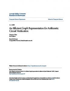
We first study our approach with different values of k. Table 3(b) shows 8 different alternatives of our method over the EU graph using different values of k. All build on the rank structure that uses 5% of extra space [13]. The first column names the approaches as follows: 0 2 × 20 , 0 3 × 30 and 0 4 × 40 stand for the alternatives where we subdivide the matrix into 2 × 2, 3 × 3 and 4 × 4 submatrices, respectively, in every level of the tree. On the other hand, we denote 0 H − i0 the hybrid approach where we use k = 4 up to level i of the tree, and then we use k = 2 for the rest of the levels. The second and third columns indicate the size, in bytes, used to store the tree T and the leaves L, respectively. The fourth column shows the space needed in main memory by the structures (e.g., including the extra space for rank), in bits per edge. Finally, the last two columns show the times to retrieve the direct (fifth column) and reverse (sixth) neighbors, measured in microseconds per link retrieved (µs/e). Note that, when we use a fixed k, we obtain better times when k is greater, because we are shortening the height of the tree, but the compression ratio worsens, as the space for L becomes dominant and many 0s are stored in there. If we use a hybrid approach, we can maintain a compression ratio close to that obtained by the 0 2 × 20 alternative while improving the time, until we get close to the 0 4 × 40 alternative. The best compression is obtained for 0 H − 30 , even better than 0 2 × 20 . Figure 3(c) shows similar results graphically, for the three larger graphs, space on the left and time to retrieve direct neighbors on the right. The space does not worsen much if we keep k = 4 up to a moderate level, whereas times improve consistently. A medium value, say switching to k = 2 at level 7, looks as a good compromise. 5.2
Comparison with other methods
We first compare graph representations that allow retrieving both direct and reverse neighbors. Figure 3(d) shows the space/time tradeoff for retrieving direct and reverse neighbors, over the larger graph (UK), as it is representative of the common behaviour of the other smaller graphs. We measure the average time efficiency in µs/e as before. Representations providing space/time tuning parameters appear as a line, whereas the others appear as a point. We compare our compact representations with the proposal in [9, Chapter 7] that computes both direct and reverse neighbors (RePair both), as well as the simpler representation in [10] (as improved in [9, Chapter 6], RePair) that retrieves just direct neigbors. In this case we represent both the graph and its
k2 -trees for Compact Web Graph Representation (a) Description of the graphs used.
(b) Different approaches over graph EU.
File
Pages Links Size (millions) (millions) (MB) CNR (2000) 0.325 3.216 14 EU (2005) 0.862 19.235 77 Indochina (2004) 7.414 194.109 769 UK (2002) 18.520 298.113 1,208
Variant 2×2 3×3 4×4 H−1 H−3 H−5 H−7 H−9
Tree (bytes) 6,860,436 5,368,744 4,813,692 6,860,432 6,860,412 6,864,404 6,927,924 8,107,036
Leaves (bytes) 5,583,076 9,032,928 12,546,092 5,583,100 5,583,100 5,583,100 5,583,100 5,583,100
Space (Hybrid approach) 6
Direct Reverse (µs/e) (µs/e) 2.56 2.47 1.78 1.71 1.47 1.42 2.78 2.62 2.67 2.49 2.39 2.25 2.10 1.96 1.79 1.67
Speed (Hybrid approach) eu indochina uk
20 time (microsec/edge)
space (bits/edge)
Space (bpe) 5.21076 6.02309 7.22260 5.21077 5.21076 5.21242 5.23884 5.72924
25
eu indochina uk
5.5
9
5 4.5 4
15
10
5
3.5 3
0 0
2
4
6 level of change
8
10
12
0
2
4
6 level of change
8
10
12
(c) Space/time behavior of the hybrid approach varying the level where we change k. UK - Direct Neighbors 25
15
2x2 3x3 4x4 Hybrid5 Hybrid37 WebGraph x 2 WebGraph x 2 (RAM) RePair x 2 RePair_both
20 time (microsec/edge)
20 time (microsec/edge)
UK - Reverse Neighbors 25
2x2 3x3 4x4 Hybrid5 Hybrid37 WebGraph x 2 WebGraph x 2 (RAM) RePair x 2 RePair_both
10
5
15
10
5
0
0 4
4.5
5
5.5
6 6.5 7 space (bits/edge)
7.5
8
8.5
4
4.5
5
5.5
6 6.5 7 space (bits/edge)
7.5
8
8.5
(d) Space/time to retrieve direct and reverse neighbors. EU - Direct Neighbors 5
time (microsec/edge)
(f) Comparison with approach Smaller.
2x2 3x3 4x4 Hybrid5 Hybrid37 WebGraph WebGraph (RAM) RePair
4
3
Space (bpe) Smaller Smaller × 2 Hybrid5 CNR 1.99 3.98 4.46 EU 2.78 5.56 5.21 Time (ms/p) CNR 2.34 0.048 EU 28.72 0.099
2
1
0 4
5
6
7
8
9
space (bits/edge)
(e) Retrieving only direct neighbors. Fig. 3. Experimental evaluation
10
Nieves R. Brisaboa, Susana Ladra, and Gonzalo Navarro
transpose, in order to achieve reverse navigation as well (RePair × 2). We do the same with Boldi and Vigna’s technique [6] (WebGraph), as it also allows for direct neighbors retrieval only (we call it WebGraph × 2 when we add both graphs). As this technique uses less space on disk than what the process needs to run, we show in WebGraph (RAM) the minimum space needed to run (yet we keep the best time it achieves with sufficient RAM space). All the implementations were provided by their authors. We include our alternatives 2 × 2, 3 × 3, 4 × 4, and Hybrid5, all of which use the slower solution for rank that uses just 5% of extra space [13], and Hybrid37, which uses the faster rank method that uses 37.5% extra space on top of T . As we can see, our representations (particularly Hybrid5 and 2 × 2) achieve the best compression (3.3 to 5.3 bpe, depending on the graph, 4.22 for graph UK) among all the techniques that provide direct and reverse neighbor queries. The only alternative that gets somewhat close is RePair both, but it is much slower to retrieve direct neighbors. For reverse neighbors, instead, it is an interesting alternative. Hybrid37 offers relevant tradeoffs in some cases. Finally, WebGraph × 2 and RePair × 2 offer very attractive time performance, but they need significantly more space. As explained, using less space may make the difference between being able of fitting a large Web graph in main memory or not. If, instead, we wished only to carry out forward navigation, alternatives RePair and WebGraph become preferable in most cases. Figure 3(e), however, shows graph EU, where we still achieve significantly less space than WebGraph. We also compare our proposal with the method in [2] (Smaller). As we do not have their code, we ran new experiments on a Pentium IV of 3.0 GHz with 4 GB of RAM, which resembles better the machine used in their experiments. We used the smaller graphs, on which they have reported experiments. Table 3(f) shows the space and average time needed to retrieve the whole adjacency list of a page, in milliseconds per page. As, again, their representation cannot retrieve reverse neighbors, Smaller × 2 is an estimation of the space they would need to represent both the normal and transposed graphs. Our method is orders of magnitude faster to retrieve an adjacency list, while the space is similar to Smaller × 2. The difference is so large that it could be possible to be competitive even if part of our structure (e.g. L) was in secondary memory (in which case our main memory space would be similar to just Smaller).
6
Extended functionality
While alternative compressed graph representations [6, 10, 2] are limited to retrieving the direct, and sometimes the reverse, neighbors of a given page, and we have compared our technique with those in these terms, we show now that our representation allows for more sophisticated forms of retrieval than extracting direct and reverse neighbors. First, in order to determine whether a given page p points to a given page q, most compressed (and even some classical) graph representations have no choice but to extract all the neighbors of p (or a significant part of them) and see if q is in the set. We can answer such query in O(logk n) time, by descending to
k2 -trees for Compact Web Graph Representation
11
exactly one child at each level of the tree. More precisely, at level ` we descend to child k · bp/k h−`−1 c + bq/k h−`−1 c, if it is not a zero, and compute the relative position of cell (p, q) in the submatrix just as in Section 3.3. If we arrive at the last level and find a 1 at cell (p, q), then there is a link, otherwise there is not. A second interesting operation is to find the direct neighbors of page p that are within a range of pages [q1 , q2 ] (similarly, the reverse neighbors of q that are within a range [p1 , p2 ]). This is interesting, for example, to find out whether p points to a domain, or is pointed from a domain, in case we sort URLs in lexicographical order. The algorithm is similar to Direct and Reverse in Section 3.3, except that we do not enter all the children 0 ≤ j < k of a row (or column), but only from bq1 /k h−`−1 c ≤ j ≤ bq2 /k h−`−1 c (similarly for p1 to p2 ). Yet a third operation of interest is to find all the links from a range of pages [p1 , p2 ] to another [q1 , q2 ]. This is useful, for example, to extract all the links between two domains. The algorithm to solve this query indeed generalizes all of the others we have seen. This gives times of O(n) for retrieving direct and reverse neighbors (we made a finer average-case analysis in Section 3.3), O(p2 −p1 +logk n) or O(q2 −q1 +logk n) for ranges of direct or reverse neighbors, and O(logk n) for queries on single links.
7
Conclusions
We have introduced a compact representation for Web graphs that takes advantage of the sparseness and clustering of their adjacency matrix. Our representation enables efficient forward and backward navigation in the graph (a few microseconds per neighbor found) within compact space (about 3 to 5 bits per link). Our experimental results show that our technique offers an attractive space/time tradeoff compared to the state of the art. Moreover, we support queries on the graph that extend the basic forward and reverse navigation. More exhaustive experimentation and tuning is needed to exploit the full potential of our data structure, in particular regarding the space/time tradeoffs of the hybrid approach. We also plan to research and experiment more in depth on the extended functionality supported by our representation. The structure we have introduced can be of more general interest. It could be fruitful, for example, to generalize it to binary relations, such as the one relating keywords with the Web pages, or more generally documents, where they appear. Then one could retrieve not only the Web pages that contain a keyword, but also the set of keywords present in a Web page, and thus have access to important summarization data without accessing the page itself. Our range search could permit searching within subcollections or subdirectories. Our structure could become a relevant alternative to the current state of the art in this direction, e.g. [3, 9]. Another example is the representation of discrete grids of points, for computational geometry applications or geographic information systems.
References 1. M. Adler and M. Mitzenmacher. Towards compressing Web graphs. In Proc. 11th DCC, pages 203–212, 2001.
12
Nieves R. Brisaboa, Susana Ladra, and Gonzalo Navarro
2. Y. Asano, Y. Miyawaki, and T. Nishizeki. Efficient compression of web graphs. In Proc. 14th COCOON, LNCS 5092, pages 1–11, 2008. 3. J. Barbay, M. He, I. Munro, and S. S. Rao. Succinct indexes for strings, binary relations and multi-labeled trees. In Proc. 18th SODA, pages 680–689, 2007. 4. D. Benoit, E. Demaine, I. Munro, R. Raman, V. Raman, and S. S. Rao. Representing trees of higher degree. Algorithmica, 43(4):275–292, 2005. 5. K. Bharat, A. Broder, M. Henzinger, P. Kumar, and S. Venkatasubramanian. The Connectivity Server: Fast access to linkage information on the Web. In Proc. 7th WWW, pages 469–477, 1998. 6. P. Boldi and S. Vigna. The WebGraph framework I: Compression techniques. In Proc. 13th WWW, pages 595–601. ACM Press, 2004. 7. A. Broder, R. Kumar, F. Maghoul, P. Raghavan, S. Rajagopalan, R. Stata, A. Tomkins, and J. Wiener. Graph structure in the Web. Journal of Computer Networks, 33(1–6):309–320, 2000. Also in Proc. 9th WWW. 8. H.-L. Chan, W.-K. Hon, T.-W. Lam, and K. Sadakane. Compressed indexes for dynamic text collections. ACM Transactions on Algorithms, 3(2):article 21, 2007. 9. F. Claude. Compressed data structures for Web graphs. Master’s thesis, Dept. of Comp. Sci., Univ. of Chile, August 2008. Advisor: G. Navarro. TR/DCC-2008-12. 10. F. Claude and G. Navarro. A fast and compact Web graph representation. In Proc. 14th SPIRE, LNCS 4726, pages 105–116, 2007. 11. D. Donato, S. Millozzi, S. Leonardi, and P. Tsaparas. Mining the inner structure of the Web graph. In Proc 8th WebDB, pages 145–150, 2005. 12. R. Geary, N. Rahman, R. Raman, and V. Raman. A simple optimal representation for balanced parentheses. Theoretical Computer Science, 368(3):231–246, 2006. 13. R. Gonz´ alez, S. Grabowski, V. M¨ akinen, and G. Navarro. Practical implementation of rank and select queries. In Poster Proc. 4th WEA, pages 27–38, 2005. 14. G. Jacobson. Space-efficient static trees and graphs. In Proc. 30th FOCS, pages 549–554, 1989. 15. J. Jansson, K. Sadakane, and W.-K. Sung. Ultra-succinct representation of ordered trees. In Proc. 18th SODA, pages 575–584, 2007. 16. J. Kleinberg, R. Kumar, P. Raghavan, S. Rajagopalan, and A. Tomkins. The Web as a graph: Measurements, models, and methods. In Proc. 5th COCOON, LNCS 1627, pages 1–17, 1999. 17. J. Larsson and A. Moffat. Off-line dictionary-based compression. Proc. IEEE, 88(11):1722–1732, 2000. 18. I. Munro. Tables. In Proc. 16th FSTTCS, LNCS v. 1180, pages 37–42, 1996. 19. I. Munro and V. Raman. Succinct representation of balanced parentheses and static trees. SIAM Journal on Computing, 31(3):762–776, 2001. 20. S. Raghavan and H. Garcia-Molina. Representing Web graphs. In Proc. 19th ICDE, page 405, 2003. 21. K. Randall, R. Stata, R. Wickremesinghe, and J. Wiener. The LINK database: Fast access to graphs of the Web. Technical Report 175, Compaq SRC, 2001. 22. H. Samet. Foundations of Multidimensional and Metric Data Structures. Morgan Kaufmann Publishers Inc., 2006. 23. T. Suel and J. Yuan. Compressing the graph structure of the Web. In Proc. 11th DCC, pages 213–222, 2001. 24. J. Vitter. External memory algorithms and data structures: dealing with massive data. ACM Computing Surveys, 33(2):209–271, 2001. (Version revised at 2007).