2058
IEEE TRANSACTIONS ON AUTOMATIC CONTROL, VOL. 55, NO. 9, SEPTEMBER 2010
Kalman Filter Implementation With Improved Numerical Properties Mohinder S. Grewal, Senior Member, IEEE, and James Kain
Abstract—This paper presents a new form of Kalman filter-the sigmaRho filter-useful for operational implementation in applications where stability and throughput requirements stress traditional implementations. The new mechanization has the benefits of square root filters in both promoting stability and reducing dynamic range of propagated terms. State standard deviations and correlation coefficients are propagated rather than covariance square root elements and these physically meaningful statistics are used to adapt the filtering for further ensuring reliable performance. Finally, all propagated variables can be scaled to predictable dynamic range so that fixed point procedures can be implemented for embedded applications. A sample problem from communications signal processing is presented that includes nonlinear state dynamics, extreme time-variation, and extreme range of system eigenvalues. The sigmaRho implementation is successfully applied at sample rates approaching 100 MHz to decode binary digital data from a 1.5-GHz carrier. Index Terms—Extended Kalman filter, sigmaRho Kalman filter, square root Kalman filter.
I. INTRODUCTION
T
HE Kalman filter’s [1] generalized model-based approach to optimal estimation would appear to be ideal for accelerating the transition from a conceptual definition of an estimation problem to its final algorithm implementation—bypassing the selection and testing of alternative suboptimal designs. This has not been the case for engineering disciplines such as communications and speech processing. We offer two reasons. Kalman filter robustness issues remain even after over 30 years of refining the details of implementation. Also, processing speed for Kalman filter solutions cannot approach the many-MHz update cycle times demanded for modern signal processing algorithms. In this paper, we present a new mechanization of the Kalman filter that mitigates these handicaps. Numerical stability issues of the Kalman filter were well known from the early days of Kalman filter applications-the very optimality of the estimation process suggests sensitivity to various errors. Simon [2] summarizes widely implemented solutions for these stability issues as: “ 1) increase arithmetic precision; 2) some form of square root filtering; 3) symmetrize the covariance matrix at each step; 4) initialize the covariance Manuscript received May 04, 2008; revised January 24, 2009; accepted December 12, 2009. First published February 17, 2010; current version published September 09, 2010. Recommended by Associate Editor I.-J. Wang. M. S. Grewal is with the Department of Electrical Engineering, California State University, Fullerton CA 92834 USA (e-mail:
[email protected]). J. Kain is with GeoVantage, Inc, Peabody, MA 01960 USA (e-mail:
[email protected]). Color versions of one or more of the figures in this paper are available online at http://ieeexplore.ieee.org. Digital Object Identifier 10.1109/TAC.2010.2042986
appropriately to avoid large changes; 5) use a fading memory filter; and 6) use fictitious process noise”. All recent Kalman filter instructional texts, such as [2]–[4], as well as early instructional texts [5], offer significant discussion of these issues but stop short of suggesting universal solutions. For example, multiple examples of preventing filter divergence are provided in [3] showing how injection of fictitious process noise prevents Kalman gains from approaching zero and thereby stabilizing the otherwise divergent solution—but strategies for selecting the fictitious noise characteristics are not discussed. Similarly, [4] provides extensive material covering various possible numerical issues as well as a suite of candidate solutions-but stops short of offering a generally applicable implementation approach. This paper proposes such a generalized approach where non-problem-specific thresholds are used to control the overall sensitivity of the solution. Improvement of Kalman filter execution speed has received less scrutiny although texts such as [4] provide detailed descriptions of good Kalman filter programming methods and their computational burden in terms of floating point operations. The scaling methods proposed here used to enhance robustness have the natural benefit for allowing mechanization into fixed point arithmetics—thereby offering methods for transitioning a design to high-speed digital signal processors. The thrust of this paper is to offer paths for more generalized robustness as well as accelerated throughput gained from fixed point arithmetics. To demonstrate our new approach, we address a communications problem where 74-MHz sampling is used to decode binary data from a 1.5-GHz carrier. The covariance matrix must be symmetric and positive-definite; otherwise it cannot represent valid statistics for state vector components. It was recognized during the early years of Kalman filter applications that factored-form Kalman filters (square root filters) are the preferred implementation for applications demanding high operational reliability [6]–[9]. Factored terms of the covariance matrix are propagated forward between measurements and updated at each measurement. The covariance matrix, reformed by multiplying its factors together, is ensured to be positive-semi-definite. Numerical comparison of several factored forms of the Kalman filter are described in [10]; derivations and software implementation detail for various factoredform filter variations are provided in [4]. One widely used factored form Kalman filter is the filter. The covariance matrix is defined in terms of the matrix factors and as (1) The Kalman filter form, and others described in [4], has worked well and specialized digital implementations have
0018-9286/$26.00 © 2010 IEEE
GREWAL AND KAIN: KALMAN FILTER IMPLEMENTATION WITH IMPROVED NUMERICAL PROPERTIES
been developed so that processing times for factored covariance filters are nearly the same as for traditional covariance propagation methods [4]. The individual terms of the covariance matrix can be interpreted as (2) where is the entry of the covariance matrix, is the state component, standard deviation of the estimate of the is the correlation coefficient between and state and and contain important physical inforcomponent. Both mation defining the progress of Kalman filter estimation—both in terms of the current success of estimation as well as the likelihood of future numerical issues. However, the individual terms within matrices propagated for factored form filters have no useful physical interpretation unless the covariance matrix, and in turn the statistical parameters in (2), are computed. The Kalman filter is optimal under assumptions that the model is correct and thus can exhibit intolerance to model error. Also, initial (pre-estimation) state values may be completely unknown, leading to assigning crude estimates for initial states with associated large initial standard deviations. Moreover, initial state correlations are often unknown and assumed to be zero. Such expedient initial conditions often lead to extreme initial transient behavior and early filter failure. A class of adaptive Kalman filter methods has been used to address impacts of modeling uncertainty [11]–[14]. Filter real-time performance is evaluated using residual tests with the process noise and/or measurement noise increased if the residual variance is observed to be outside the expected range. However, because the closed adaptation loop must be slower than the estimator response time, the filter may have become unrecoverable after the point the divergence is noticed. A method that can anticipate future anomalous performance is preferable. One such approach is to recognize that instability often results from extracting too much information too quickly from the estimation process. A slower rate of convergence and/or limiting the lower threshold of the estimate standard deviation would be preferable to potential divergence. One method to achieve this result is to compute the Kalman filter updated covariance with the physics-based model parameters and test the resulting covariance matrix. If too much estimate improvement is predicted, then either the measurement noise or the process noise levels can be increased and the covariance update recomputed before processing the data at this step. Such an iterative procedure leads to a limited information filter where the maximum standard deviation improvement (per measurement) for any state is limited. In a similar way, we could limit the lower extent of a state standard deviation to an absolute value or to a percentage of its original uncertainty level. The difficulties of such adaptive approaches are primarily computational. A filter form could readily be devised to cycle through the covariance update computations, iteratively adjusting noise models to limit the information extraction. Fading memory filters [2], [15], [16] are also offered as generalized solutions for mitigating divergence tendencies. These filters de-weight less recent data, forcing the filter to always accept new information, thus preventing Kalman gains
2059
from approaching zero. However, as with adding fictitious process noise, this stabilizing solution must use trial-and-error methods to tune the manner in which prior measurement data is de-weighted. The computer word length issues that plagued early Kalman filter implementations have been somewhat mitigated by the power of today’s computers. However, Kalman filter solutions rarely receive consideration for extreme speed embedded applications such as communications, speech and video data processing where fixed point solutions are preferred. This paper derives an alternative Kalman filter mechanization with direct propagation of the standard deviation (sigma) and correlation (Rho) matrix that we call the sigmaRho filter. This new filter form offers a more generalized solution to the numerical issues of the Kalman filter described above. The new filter offers an added benefit in that its internal numerical values are naturally scaled in a manner so that a fixed point implementation is straightforward. Section II derives the sigmaRho filter for nonlinear continuous and discrete systems, the measurement update step, and the adaptation strategy. Section III presents an example of the fixed point sigmaRho filter applied to a communications problem, and Section IV gives the conclusions. II. A NEW KALMAN FILTER MECHANIZATION FOR CONTINUOUS NON-LINEAR SYSTEMS A. The System Dynamics For a Kalman filter, the system state differential equations are given by (3) where state variable vector of length ; state dynamics, often linearized with ; system white noise vector inputs with . The scalar measurement process is described by (4) where scalar measurement value; measurement model, often linearized by ; measurement noise with . There is no loss of generality by treating only scalar measurements. The scalar measurement model is equivalent to an -vector measurement model under conditions where the measurements are uncorrelated (diagonal matrix ). For this case, each of the measurements is processed sequentially at a single measurement epoch. Moreover, correlated measurements contains off-diagonal elements) can be decomposed into ( an equivalent uncorrelated representation with a net benefit in execution time over direct inclusion of a non-diagonal matrix through matrix inversion [4].
2060
IEEE TRANSACTIONS ON AUTOMATIC CONTROL, VOL. 55, NO. 9, SEPTEMBER 2010
B. The SigmaRho Filter Covariance and State Propagation With Continuous Dynamics The estimation problem description is frequently based on a continuous linear or nonlinear differential equation with the general form of (3). The continuous dynamic state estimate and its covariance matrix must be transitioned from a measurement epoch to the next measurement epoch. This transition process can be accomplished by a simple trapezoidal integration of the continuous filter dynamics when measurement sample times are fast with respect to system dynamics. For linear or linearizable systems, matrix exponential solutions are often used to transform the continuous system to a discrete form using the transition matrix. For system models that do not fall into either of these categories, direct numerical integration of nonlinear continuous differential equations can provide an effective solution. The discrete form is discussed in Section II-C. The state propagation step between measurements for the Kalman filter is governed by (5)
vectors are large. Thus the summation in (13) might require considerable multiples by zero or one; otherwise some sparse matrix logic must be added to bypass these multiplies. However, the general expression , where is an arbitrary vector quantity, is easily computed using a problem-specific procedure with a vector quantity result. Numerical methods that capitalize on this form of sparse matrix treatment are referred to as Krylov techniques [17]. We introduce the following equation as an aid to avoid specialized sparse matrix logic
(14) Thus (13), scaled with
to remove physical units, becomes (15)
We return to the more general case where and (11) gives the following result:
. Using (9)
We consider a scaling of this state vector as follows: (16)
(6) component of the state vector and where is the instantaneous (time varying) standard deviation of the vector component. Thus, we can write
is the state
Solving for
gives (17)
(7) Equation (7) provides the dynamics for the transformed state vector . Covariance propagation for a continuous linear or linearized dynamic system is governed by (8) Taking the time derivative of (2) (9) We first investigate the terms of this equation where and are identical. Noting that and , then, from (9) (10) From (8) expressed in scalar form (11) and, substituting from (10) and setting (12)
The standard deviation in the propagation step (15) is the only statistical term that is not scaled. The standard deviation has the same physical units as the original states and may have large dynamic range depending on the engineering model. Dividing by a pre-defined maximum expected value (unique for each state) can normalize the standard deviation derivatives. It is often the case that the initial state standard deviation is set to its maximum expected value over time with the subsequent standard deviations improved by the estimation process. Table I shows the final propagation equations when all statistic variables are scaled to predictable ranges. The subscripted terms are the state-specific maximum standard deviation values and the primed standard deviation terms are the normalized terms (expected to be between 0 and 1). The attention to normalization not only promotes numerical stability but, as we shall demonstrate later, enables a straightforward transition to a fixed point implementation. C. The SigmaRho Filter Covariance and State Propagation With Discrete Dynamics Often it is desirable to recast a continuous dynamic system into a discrete form for state propagation from epoch to epoch using the transition matrix and discrete noise using
Equation (12) reduces to the simple form
(18) (13)
We introduce an auxiliary variable that aids the computational process. The matrix is often sparse, particularly when state
Covariance propagation is performed by (19) where
.
GREWAL AND KAIN: KALMAN FILTER IMPLEMENTATION WITH IMPROVED NUMERICAL PROPERTIES
TABLE I SIGMARHO PROPAGATION FOR CONTINUOUS SYSTEM DYNAMICS
2061
TABLE II SIGMARHO PROPAGATION FOR DISCRETE SYSTEM DYNAMICS
For the discrete sigmaRho form, we begin by normalizing the state vector at the beginning of each propagate step
We also must update the state between measurements. The update to account for the transformed state is performed by (26)
(20) where is the standard deviation value for the ponent after the last measurement update. We will define
state com-
(21) Note that
The state is normalized by its standard deviation and the correlation coefficients are naturally normalized to between . However, as for the continuous case, the standard deviation dynamic range may vary significantly among states for a specific problem. As before, we use the normalization (27) is the maximum expected value of the state where standard deviation. The normalized state dynamics use transformations
(22) We propagate the covariance matrix of the normalized system from the last measurement to the next measurement, noticing from (22) that the covariance matrix of the normalized system is just the correlation matrix after the prior measurement (23) where . The “ ” superscript represents values immediately after the last measurement and the “ ” superscript indicates the value at the next measurement but before the measurement update processing. From (22) and (23), it can be seen that (24)
(28) (29) Note that (24), (25) and (26) that propagate the standard deviation, correlation matrix, and state, respectively, all use only ratios of the standard deviation change between measurements. Therefore, these computations do not change as a result of the time-invariant scaling of (27). The states are normalized by their individual standard deviations. This strategy deems the various states unitless, potentially reducing dynamic range; however, there may remain a large state dynamic range for states that have a large physical variation with small estimate standard deviation. Further state estimate scaling by a constant, , applied to all states, can be useful and requires no modification of the propagation equations. The final normalized state estimate is (30)
and (25)
The final propagation equations for the discrete dynamics are provided in Table II.
2062
IEEE TRANSACTIONS ON AUTOMATIC CONTROL, VOL. 55, NO. 9, SEPTEMBER 2010
D. The SigmaRho Filter State and Covariance Update at a Measurement
Now we must perform the covariance update computation. Using subscripts, (32) becomes
The covariance update process for traditional Kalman filters uses the equations (31) (32) where
(41) Substituting the sigma and rho notation, (41) becomes (42)
is the Kalman gain used in the following manner (33)
with variables and represented as scalars without loss of generality [4]. We begin to decompose (31) and (32) by introducing the subscript notation and the sigma and rho terms as before. Thus, we can form the expression
Using the
auxiliary notation gives (43)
and inserting the definition of the Kalman gain (44)
(34) As with the auxiliary parameters used in the covariance propagation, sparse matrix procedures can be avoided by using the terms (35)
Equation (44) is a general expression for an arbitrary entry of the covariance matrix. Restricting the computation to the diagonal entries gives (45) Now, solving for the standard deviation improvement ratio across a measurement
Thus, (34) becomes (36) Continuing this theme to develop the terms from (31) (37)
(46) At this point, we return to the general expression, (44). Solving this expression for the new correlation coefficient after the measurement gives (47)
and finally (38)
The non-normalized state update at the measurement sample period is given by (48)
We introduce an additional variable (39) that is useful for normalization of the residual term. In this expression, is the standard deviation of the residual process. An excellent measure of performance of a Kalman filter is the whiteness of the residual time sequence and the containment of the residuals within the one-sigma residual bound defined by . The Kalman gain is formed by (40)
Note the impact on (48) of using state normalization factors. Divide both sides by the standard deviation before measurement and multiply both sides by . We must also renormalize the in preparation for the state to the new standard deviation, next propagation step so that, finally (49) Equation (49) summarizes the sigmaRho Kalman filter state update. However, we have used a normalized standard deviation during the continuous and discrete propagate steps. Fortunately,
GREWAL AND KAIN: KALMAN FILTER IMPLEMENTATION WITH IMPROVED NUMERICAL PROPERTIES
2063
term beneath the radical in (46): The scalar quantity can take any value, provided that the following constraint is maintained:
TABLE III DISCRETE SIGMARHO FILTER MEASUREMENT UPDATE
(51) . where Using the above definition for in (46), we see that the standard deviation update ratio is given by (52) The term on the left must be between 0 and 1 with 1 being no improvement from the measurement and 0 being a non-realizable improvement to zero standard deviation. As the term on the left approaches 0, the filter tends to become unstable. Thus we can define (53) the update processing mathematics requires ratios of the standard deviations in all cases except for the computation of the residuals. We can define a normalized measurement matrix as (50) With this definition we can express the final measurement update process as in Table III. The primed standard deviation terms correspond to the normalized standard deviations that will have predictable dynamic range for use in a fixed point implementation. E. SigmaRho Filter Adaptation One of the benefits of the SigmaRho filter is the ready availability of the standard deviation and correlation coefficient statistics for use in monitoring the filter performance. However, monitoring the performance is not sufficient to prevent numerical ill-conditioning. We must both monitor and control these statistics before they attain meaningless values (i.e., negative ). There are two standard deviations or correlations outside user-defined noises that are available for controlling the standard deviations and correlation coefficients: measurement noise and process noise. The process noise is typically more useful for adaptation because: 1) process noise is often more uncertain than measurement noise; 2) added process noise elevates the steady state performance (often desirable to the designer); and 3) process noise can be used to more surgically control issues that are posed by single states within the model without interfering with other states that may be well-behaved. Alternatively, measurement noise adaptation is particularly useful during the initial startup stage of the Kalman filter. We will first discuss our adaptation using measurement noise and then describe adaptation using process noise. Initial state estimates, before any measurement processing, are sometimes assumed to be completely unknown, suggesting an infinite standard deviation. Computationally, this policy is implemented by setting the initial standard deviations to a large number. Also, state correlations are often assumed to be zero. The initial transient numerical issues almost always result from the update step. A key observation can be made by inspecting the
is the desired lower limit value for . where Setting to a higher value (closer to 1), results in a more stable filter with less reduction in the post-update standard deviations. We can compute the effective measurement variance for a given value of as (54) Thus selecting a value for can be considered as a mechanism for adapting the scalar measurement noise . However, it is important to note that being above 1.0 does not ensure a positive value for . However, need not be computed using (54). In fact, it is not numerically desirable to compute because the squaring of the terms on the right of (54) spreads the dynamic range of computed variables. From Table III, we see that (55) For the important initial transient period, the first term on the right of (55) is typically much larger than the measurement variance and is reduced through the course of the initial estimation values are reduced. We have observed benefits from as the the following conservative approximation: (56) . so that The assumption of (56) is exact if H has only a single nonand zero term. With the approximation (56), we can monitor trigger the measurement noise adaptation only when
The adaptation using measurement noise described in this section has the following benefits: easily implemented in software, will not promote covariance matrix indefiniteness, reduces dynamic range of computed variables, and is well suited
2064
IEEE TRANSACTIONS ON AUTOMATIC CONTROL, VOL. 55, NO. 9, SEPTEMBER 2010
for treating frequently encountered initial transient instability issues. Next consider the adaptation using the process noise. The key drawback of adaptation using measurement noise is that this penalizes all states where only a single state may be problematic. Insertion of process noise can be used to better target individual state estimation issues within a complex large-scale problem. Consider the following covariance matrix modification
is the sinusoidal signal output. The covariance matrix where is given by
(65) with steady state solution
given by
(57) where is a diagonal matrix with each diagonal term having the effect of adding process noise to an individual state. We see that (58) and (59) Now let
(66) Using this stochastic model with a low value for damping generates a near-constant frequency signal so that the signal spectrum peaks near the indicated frequency. If we set the model output variance to unity ( is equal to one), then we can create a representation of a single-frequency tone with RMS amplitude of one. The degree of prescribed stochastic variability (amplitude and phase) for this model can be used to represent realworld communication signal uncertainties. The transition matrix for this system is given by [4]
(60) so that (61) (67) (68)
(62) Equations (61) and (62) provide a simple but statistically-correct way to compute to adapt the process noise to prevent individual state estimate standard deviations from getting too small . or individual correlation coefficients getting too close to In this manner, we can anticipate the onset of stressful numerical situations and take action to prevent them from occurring. Equations (61) and (62) must be performed together to ensure positive-definiteness of the covariance matrix.
The Power Spectral Density (PSD) [4] is given by (69) The autocorrelation [4] of the near-sinusoidal response is (70)
III. APPLICATION TO SIGNAL PROCESSING We demonstrate here how the sigmaRho filter can be applied to a communication problem: estimation of information modulated onto a noisy carrier waveform. We use a linear secondorder system to represent a highly coherent sinusoidal signal with the degree of coherence (ability to predict forward in time) adjusted with a design parameter. The represented carrier signal has uncertain amplitude as well as an uncertain component to its frequency. The carrier is modulated with digital information using Binary Phase Shift Key (BPSK) encoding resulting in phase shifts of 180 at the data encoding rate. The carrier waveform is directly sampled at a rate well below the carrier frequency but faster than the encoding rate. A sinusoidal signal with frequency can be represented as . An oscillator can a second order system with low damping be represented by the following differential equation: (63) or, using state-space notation (64)
We see from Fig. 1 how the model can be adjusted to represent any degree of single-frequency signal coherence. For example, , a signal value we see for damping of 0.0001 and 100 cycles forward in time is correlated to the current signal value with a correlation coefficient of 0.90. The communications sample problem is formed from two interconnected second-order systems as shown in Fig. 2. One of the second order systems represents a highly coherent single frequency carrier and the second second-order low pass system represents an unknown frequency component of the carrier. The digital sample rate of the carrier is chosen to be much lower than the carrier frequency. Finally, the phase of the carrier will be changed instantaneously to represent a BPSK digital data encoding (Fig. 3). The objective is to estimate the uncertain carrier frequency and, simultaneously, estimate the phase transitions to recover the encoded data. The nonlinear state dynamics are given by (71), shown at the bottom of the low pass frequency uncertainty next page, where sinusoidal carrier model with output , and state represents the carsignal model with output . The rier-plus-information signal to be measured.
GREWAL AND KAIN: KALMAN FILTER IMPLEMENTATION WITH IMPROVED NUMERICAL PROPERTIES
2065
Fig. 3. Binary phase shift key (BPSK) data encoding represented as two model classes.
Note the coupling between the mean state and covariance propagation as represented by the state-dependent system main the third row, second column of trix. The term is a particular issue because it is both large in magnitude and rapidly time-varying between measurements. The continuous system noise matrix is given by
Fig. 1. Autocorrelation of near-sinusoidal carrier model.
(74)
where the diagonal terms result from the steady state solutions for the two second order systems as given by (66). The measurement model for the Kalman filter is Fig. 2. Uncertain carrier model formed from two second order linear processes.
The continuous nonlinear system propagation between measurements is given by
(75) A closed form solution for the transition matrix, obviating the need for solving the matrix exponential or use of numerical integration techniques, is the key to high-speed embedded Kalman filter applications. For the communications problem, we can write the general form of the 4 4 transition matrix as
(72) (76) The dynamics matrix for covariance propagation between measurements is given by (73), shown at the bottom of the page.
The 2 2 sub-matrices and along the diagonal will be defined from the transition matrix for second order systems (67) with appropriate damping and frequency, noting that
(71)
(73)
2066
IEEE TRANSACTIONS ON AUTOMATIC CONTROL, VOL. 55, NO. 9, SEPTEMBER 2010
the frequency error varies slowly with respect to the sample time and is a small fraction of the carrier frequency. The top right entry is zero because the carrier signal model does not influence the frequency error model. The lower left entry reflects the effect of the frequency error on the future composite signal and requires careful consideration. We can derive an approxiby recognizing that mation to
We can write (77) Our transition matrix for the carrier frequency second order is based upon assumption of a constant fresystem quency (and thus constant frequency error). We approximate using a Taylor’s expansion with the value for at the midpoint of the measurement interval. Thus
(78) Taking the partial derivative from (72) we can write
(79) Equations (77) and (78) allow computation of from paris a strong tial derivatives as indicated by (79). Note that function of the rapidly varying carrier model states as expected for the nonlinear system. We also require a closed form solution for the discrete noise matrix. Fortunately, the discrete noise matrix for a generalized second order system has been solved in closed form in [4]. The results are summarized as follows: (80) (81)
(82) (83) (84) The generalized expression for , with suitable damping and frequency, can be used for the two 2 2 sub-matrices of the discrete noise for the software radio problem. We assume that
the contribution of the frequency error stochastic dynamics to the carrier frequency model is negligible. Thus the off-diagonal 2 2 terms in the discrete noise matrix are assumed to be zero. We simulate the data encoding by modifying the phase of the perturbed carrier by 180 as illustrated in Fig. 3. The binary data detection scheme will use maximum likelihood hypothesis testing principles [18] based on the assumption of a two-class structure. The normalized residual is tested at each measure). If the threshold is ment epoch against a threshold (e.g., violated, the sign of the estimated carrier signal states, along with the correlation coefficients between the carrier states and carrier error states, are changed to represent the alternative hypothesized class with 180 phase change of the carrier. If this change brings the residual within the threshold, a phase change is assumed. That is, we detect the occurrence of an abnormal residual, modify the signal state and covariance to represent the alternative signal class for the assumed two-class model representation, and then retest the normalized residual as verification. This process is readily extended to other forms of PSK data encoding. For this example, we have used a practically useful carrier , sampled at 1/20.25 the carfrequency of 1.5 GHz rier frequency (74 MHz) with measurement noise amplitude of 10% of the carrier, and with BPSK encoding at 1/200 the carrier frequency (7.5 MHz). The perturbation carrier model assumes a . The simulated carrier frequency bandwidth of 0.1 Hz reflected as times an error is held constant at initial assumed carrier uncertainty of 100 PPM. Filter adaptation, using both measurement and process noise, as described in Section E, was used to limit the state standard deviation improvement to 50% per sample, the standard deviation floor to 10% of original uncertainty, and correlation coefficients to be . within Fig. 4 shows results for 200 000 carrier cycles for a double precision implementation of the sigmaRho filter. The top pane in Fig. 4 shows the actual noisy measurement (red) and the prediction of the measurement from the Kalman filter (blue). The middle pane shows the Kalman filter normalized residuals. The normalization factor is the Kalman filter prediction of the residual one-sigma bound-so that 68% of the data should be confor a well-performing Kalman filter. The bottom tained with pane shows the estimate of the carrier frequency error (red) and its predicted one-sigma value (blue), both in terms of improvement factor with respect to the initial uncertainty (100 PPM). The inset on Fig. 4 shows the detail of the detected BPSK coded data that was encoded as alternating zero-one. For this example, all indicators suggest the sigmaRho filter and data decoding performs as expected with 100% success of the data decoding. Next, we will illustrate the fixed-point implementation of the sigmaRho filter. The objective is that all internal filter variables can be represented by a single fixed point number format using the available sigmaRho scaling parameters. The total bits in the where is the number of bits in the fixed point format are integer part of the fixed point word and is the number of bits , in the fixed point fraction. By multiplying all variables by the add and subtract operations are handled by standard integer so that all internal math operations. The goal is that . The fraction variables are scaled to a dynamic range of bits are adjusted to maintain performance similar to the double
GREWAL AND KAIN: KALMAN FILTER IMPLEMENTATION WITH IMPROVED NUMERICAL PROPERTIES
Fig. 4. Simulation results for 1.5 GHz carrier with BPSK encoding at 7.5 MHz.
2067
Fig. 5. SigmaRho Kalman filter fixed point mechanization with 2-b mantissa and 10-b fraction.
precision implementation. In order to limit the fixed point math operations to add, subtract, multiply and divide, the square root operations were approximated using the following forms: (85)
(86) These approximated values are larger than the exact value, which results in a more conservative filter. That is, errors in these approximations tend to result in a more positive-definite covariance matrix. Implementing the fixed point math operations requires two special numerical procedures that are used to implement fixed point multiply and divide: 1) Fixed point multiply:
Fig. 6. Sigma\Rho Kalman filter fixed point mechanization with 2-b mantissa and 8-b fraction.
(87) 2) Fixed point divide: (88) , and are fixed point formatted variables where . Software converted to an integer through multiplication by can be developed to move between double precision and fixed point implementation by using a custom selectable procedure for mechanizing all multiply and divide operations. A custom floating point multiply and divide procedure is also used to track the maximum and minimum of all internally computed variables so that the required value for a fixed point mantissa (L) can be determined using either simulated processing or actual data processing using a double precision form.
For the sample problem parameters (but with the error ), we found that a 16-b fixed point switched to ) provided indistinguishable implementation results from the double precision version; moreover even further word size reduction provided stable results. Figs. 5 and 6 show the graceful degradation of the estimation result as the fixed point word length was reduced from 16 b to 12 b and then to 10 b—both with 2-b integer part. The 10-b implementation begins to show signs of deterioration; however, the ability to decode the binary data remains intact. IV. CONCLUSION The Kalman filter has enjoyed wide acceptance in complex high-end aerospace and defense applications where high-performance computers are an accepted element of the processing
2068
IEEE TRANSACTIONS ON AUTOMATIC CONTROL, VOL. 55, NO. 9, SEPTEMBER 2010
architecture. However, it is rare for the Kalman filter to receive even minimal coverage in texts describing digital signal processing techniques. In order for Kalman filtering to receive more attention as a signal processing tool for high-speed commercial applications, software designers must 1) become more confident that stable performance can be guaranteed, and 2) know there exists a generalized implementation path for fixed point digital processing hardware. This paper has presented the sigmaRho variant of the Kalman filter to address these shortcomings. The sigmaRho filter offers a fundamentally different approach to traditional stable Kalman filter forms that are based on a factored covariance matrix and/or noise adaptations based on monitoring residual processes. Factored forms mask the underlying statistical terms that can provide a preventative diagnostic, and residual-based adaptations can only react to divergence. The sigmaRho filter naturally propagates the standard deviation and correlation coefficients for all variables without added computational complexity. As a natural extension, generalized methods are readily available to both monitor and control these critical statistical parameters in a manner to promote operational stability while specifying the impact of desensitization on estimation performance. Of equal importance, the sigmaRho filter algorithm offers a normalized solution to allow the control of the dynamic range of all computational variables. This normalization, in turn, offers a straightforward path to the implementation of the sigmaRho filter using high-speed embedded digital processors.
REFERENCES [1] R. E. Kalman, “A new approach to linear filtering and prediction problems,” ASME J. Basic Eng., vol. 82, pp. 32–45, 1960. [2] D. Simon, Optimal State Estimation: Kalman, H-Infinity and Nonlinear Approaches. New York: Wiley, 2006. [3] P. Zarchan and H. Musoff, Fundamentals of Kalman Filtering: A Practical Approach, 2nd ed. Reston, VA: American Institute of Aeronautics and Astronautics, 2005, pp. 616–617. [4] M. S. Grewal and A. P. Andrews, Kalman Filtering Theory and Practice Using MATLAB, 3rd ed. New York: Wiley, 2008. [5] A. Gelb, Applied Optimal Estimation. Boston, MA: MIT Press, 1974, pp. 204–210. [6] J. E. Potter and R. G. Stern, “Statistical filtering of space navigation measurements,” in Proc. AIAA Guid. Control Conf., New York, NY, 1963. [7] N. A. Carlson, “Fast triangular formulation of the square root filter,” AIAA J., vol. 11, no. 9, pp. 1259–1265, 1973. [8] G. J. Bierman, Factorization Methods for Discrete Sequential Estimation. New York: Academic, 1977. [9] C. J. Thornton and G. J. Bierman, “Filtering and error analysis via the UDU covariance factorization,” IEEE Trans. Autom. Control, vol. AC-23, no. 5, pp. 901–907, Oct. 1978. [10] K. Lemon and B. W. Welch, Comparison of Nonlinear Filtering Techniques for Lunar Surface Roving Navigation, NASA/TM2008–215152. Cleveland, OH: Glenn Research Center, 2008. [11] M. Oussalah and J. De Schutter, “Adaptive Kalman filter for noise identification,” in Proc. ISMA25 Int. Conf. Noise Vibration, Leuven, Belgium, Sep. 13-15, 2000.
[12] R. K. Mehra, “On the identification of variance and adaptive Kalman filtering,” IEEE Trans. Autom. Control, vol. AC-15, no. 2, pp. 175–184, 1970. [13] R. K. Mehra, “Approaches to adaptive filtering,” IEEE Trans. Autom. Control, vol. AC-17, no. 5, pp. 693–698, Oct. 1972. [14] K. A. Myers and B. D. Taply, “Adaptive sequential estimation with unknown noise statistics,” IEEE Trans. Automatic Control, vol. AC-21, no. 5, pp. 520–523, Aug. 1976. [15] J. Sacks and H. Sorenson, “Nonlinear extensions of the fading memory filter,” IEEE Trans. Autom. Control, vol. AC-16, no. 5, pp. 506–507, Oct. 1971. [16] J. I. Statman, “A recursive solution for a fading memory filter from Kalman filter theory,” in Proc. NASA/JPL TDA Progress Rep. 42-86, Apr./Jun. 1986, pp. 70–76. [17] V. Druskin and Knizhnerman, “Krylov space approximations of eigenpairs and matrix functions in exact and computer Arithmetic,” Numer. Linear Algebra. APPL 2, pp. 205–217, 1995. [18] H. Akaike, “A new look at the statistical model identification,” IEEE Trans. Autom. Control, vol. 19, no. 6, pp. 716–723, Dec. 1997. Mohinder S. Grewal (M’68–SM’80) received the Ph.D. degree in electrical engineering (with a specialization in control systems and computers) from the University of Southern California, Los Angeles, in 1974. He coauthored Kalman Filtering: Theory and Practice Using MATLAB Third Edition (New York: Wiley2008) and Global Positioning Systems, Inertial Navigation, and Integration Second Edition (New York: Wiley, 2007). He has published over 65 papers in IEEE and ION refereed journals and proceedings, including the Institute of Navigation’s Redbook. He has consulted with Raytheon Systems, Boeing Company, Lockheed-Martin, and Northrop on application of Kalman filtering. Currently, he is Professor of Electrical Engineering at California State University, Fullerton, Fullerton, CA, where he received the 2009 Outstanding Professor award. He is an architect of the GEO Uplink Subsystem (GUS) for the Wide Area Augmentation System (WAAS), including the GUS clock steering algorithms, and holds two patents in this area. His current research interest is in the area of application of GPS, INS integration to navigation. Dr. Grewal received the 2009 Outstanding Professor award from the California State University, Fullerton. He is a member of the Institute of Navigation and a Fellow of the Institute for the Advancement of Engineering. GPS World Magazine named him as one of “50+ Leaders to Watch” in its May 2007 issue. He serves as a Reviewer for several IEEE publications.
James Kain received the M.S. degree from the Massachusetts Institute of Technology, Cambridge, in 1970. He has over 35 years experience in practical implementation of estimation theory and vehicle control with emphasis on navigation systems and multisensor applications. He has developed, implemented, and tested numerous Kalman filter-based solutions to practical systems problems. He has consulted with Draper Lab, Johns Hopkins Applied Physics Laboratory, and TASC (now Northrop Grumman). Since 1995, he co-founded three successful start-up ventures, including Enpoint Incorporated, where a patented short-baseline dual GPS antenna solution, coupled with a MEMS IMU, was developed for precision attitude determination. Currently, he is Executive Vice President at GeoVantage, Inc. (one of his start-ups subsequently acquired by John Deere), Peabody, MA. GeoVantage’s remote sensing technology is based upon integration of INS/GPS and digital imagery with the Kalman filter used to integrate the various sensors in a synergistic manner.