Kalman Filtering in R - Journal of Statistical Software

JSS

Journal of Statistical Software March 2011, Volume 39, Issue 2.

http://www.jstatsoft.org/

Kalman Filtering in R Fernando Tusell University of the Basque Country

Abstract Support in R for state space estimation via Kalman filtering was limited to one package, until fairly recently. In the last five years, the situation has changed with no less than four additional packages offering general implementations of the Kalman filter, including in some cases smoothing, simulation smoothing and other functionality. This paper reviews some of the offerings in R to help the prospective user to make an informed choice.

Keywords: state space models, Kalman filter, time series, R.

1. Introduction The Kalman filter is an important algorithm, for which relatively little support existed in R (R Development Core Team 2010) up until fairly recently. Perhaps one of the reasons is the (deceptive) simplicity of the algorithm, which makes it easy for any prospective user to throw in his/her own quick implementation. While direct transcription of the equations of the Kalman filter as they appear in many engineering or time series books may be sufficient for some applications, an all-around implementation requires more complex coding. In Section 2, we provide a short overview of available algorithms. It is against this background that we discuss in Section 3 the particular choices made by four packages offering fairly general Kalman filtering in R, with some mention of functions in other packages which cater to particular needs. Kalman filtering is a large topic. In the sequel we focus on linear Gaussian models and their estimation, which is what the packages we review offer in common (and the foundation on which most anything else rests). Other functionalities present in some of the packages examined include filtering and estimation of non-Gaussian models, simulation and disturbance smoothing and functions to help with the Bayesian analysis of dynamic linear models, etc. none of which are assessed.

2

Kalman Filtering in R

2. Kalman filter algorithms We shall consider a fairly general state-space model specification, sufficient for the purpose of the discussion to follow in Section 3, even if not the most comprehensive. The notation follows Harvey (1989). Let αt = ct + Tt αt−1 + Rt ηt

(1)

yt = dt + Zt αt + t

(2)

where ηt ∼ N (0, Qt ) and t ∼ N (0, Ht ). The state equation (1) describes the dynamics of the state vector αt , driven by deterministic (ct ) and stochastic (ηt ) inputs. The observation (or measurement) equation links the observed response yt with the unobserved state vector, with noise t and (possibly) deterministic inputs dt . Matrices Tt , Rt , Zt , Qt and Ht may depend on a vector of parameters, θ, and be time varying or constant over time. The noises ηt and t are assumed serially and also mutually uncorrelated, i.e., E[ηt > s ] = 0 for all t, s. The last assumption and the gaussianity of ηt and t can be dispensed with; see e.g., Anderson and Moore (1979).

2.1. The Kalman filter. The Kalman filter equations, with slight notational variations, are standard in any textbook: see, e.g., Anderson and Moore (1979), Simon (2006), Durbin and Koopman (2001), Grewal and Andrews (2001), West and Harrison (1997) or Shumway and Stoffer (2006), to name only a few. We reproduce those equations here, however, as repeated reference is made to them in the sequel. Define at−1 = E[αt−1 |y0 , . . . , yt−1 ]

(3) >

Pt−1 = E[(αt−1 − at−1 )(αt−1 − at−1 ) ]

;

(4)

estimates of the state vector and its covariance matrix at time t with information available at time t − 1, at|t−1 and Pt|t−1 respectively, are given by the time update equations at|t−1 = Tt at−1 + ct

(5)

Pt|t−1 = Tt Pt−1 Tt> + Rt Qt Rt> .

(6)

Let Ft = Zt Pt|t−1 Zt > + Ht . If a new observation is available at time t, then at|t−1 and Pt|t−1 can be updated with the measurement update equations at = at|t−1 + Pt|t−1 Zt> Ft−1 (yt − Zt at|t−1 − dt ) Pt = Pt|t−1 −

Pt|t−1 Zt Ft−1 Zt> Pt|t−1 .

(7) (8)

Equations (5)–(6) and (7)–(8) taken together make up the Kalman filter. Substituting (5) in (7) and (6) in (8), a single set of equations linking at−1 and Pt−1 to at and Pt can be obtained. In order to start the iteration we need initial values of a−1 and P−1 (or a0|−1 and P0|−1 ). The filter equations (6) and (8) propagate the covariance matrix of the state, and are said to define a covariance filter (CF). Equivalent equations can be written which propagate the matrix Pt−1 , giving an information filter (IF). Information filters require in general more

Journal of Statistical Software

3

computational effort. One possible advantage is that they provide a natural way to specify complete uncertainty about the initial value of a component of the state: we can set the corresponding diagonal term in the information matrix to zero. With a covariance filter, we have to set the corresponding variance in P0|−1 to a “large” number, or else use exact diffuse initialization, an option described below. Direct transcription of the equations making up the Kalman filter into computer code is straightforward. It was soon noticed, though, that the resulting programs suffered from numerical instability; see for instance Bucy and Joseph (1968). In particular, buildup of floating point errors in equation (8) may eventually yield non symmetric or non positive definite Pt matrices. An alternative to equation (8) (more expensive from the computational point of view) is: Pt = (I − Kt Zt )Pt|t−1 (I − Kt Zt )> + Kt Ht Kt>

(9)

with Kt = Pt|t−1 Zt> Ft−1 ; but even this (“Joseph stabilized form”, see Bucy and Joseph (1968), p. 175) may prove insufficient to prevent roundoff error degeneracy in the filter. A detailed reference describing the pitfalls associated with the numerical implementation of the Kalman filter is Bierman (1977); see also Grewal and Andrews (2001), Chap. 6 and Anderson and Moore (1979), Chap. 6. Square root algorithms, that we discuss next, go a long way in improving the numerical stability of the filter.

2.2. Square root algorithms Consider a matrix St such that Pt = St St > ; square root covariance filter (SRCF) algorithms propagate St instead of Pt with two main benefits (cf. Anderson and Moore (1979), § 6.5): (i) Re-constitution of Pt from St will always yield a symmetric non negative matrix, and (ii) The numerical condition of St will in general be much better than that of Pt . If instead of the covariance matrix we choose to factor the information matrix Pt−1 we have a square root information filter algorithm (SRIF). It is easy to produce a replacement for the time update equation (6). Consider an orthogonal matrix G such that:     > T> St−1 M t (10) =G 0 (Q1/2 )T Rt> where M is an upper triangular matrix. Matrix G can be constructed in a variety of ways, including repeated application of Householder or Givens transforms. Multiplication of the transpose of (10) by itself produces, taking into account the orthogonality of G, M >M

1/2

> = Tt St−1 St−1 Tt> + Rt Qt

=

Tt Pt−1 Tt>

+

Rt Qt Rt>

;

1/2 T

(Qt

) Rt >

(11) (12)

comparison with (6) shows that M is a possible choice for St|t−1 . Likewise, it can be shown (Simon 2006, Section 6.3.4) that the orthogonal matrix G∗ such that " #   1/2 T > > ∗ (Ht + Zt Pt|t−1 Zt ) Kt (Ht ) 0 = G∗ (13) > > 0 M∗ St|t−1 Zt> St|t−1 produces in the left-hand side of (13) a block M ∗ that can be taken as St , and thus performs the measurement update.

4

Kalman Filtering in R

Although the matrices performing the block triangularizations described in equations (10) and (13) can be obtained quite efficiently (Lawson and Hanson 1974; Gentle 2007), clearly the computational effort is greater than that required by the time and measurement updates in equations (6) and (8); square root filtering does have a cost. In the equations above G and G∗ can be chosen so that M and M ∗ are Cholesky factors of the corresponding covariance matrices. This needs not be so, and other factorizations are possible. In particular, the factors in the singular value decomposition of Pt−1 can be propagated: see for instance Zhang and Li (1996) and Appendix B of Petris et al. (2009). Also, we may note that time and measurement updates can be merged in a single triangularization (see Anderson and Moore 1979, p. 148, and Vanbegin and Verhaegen 1989).

2.3. Sequential processing In the particular case where Ht is diagonal, the components of yt > = (y1t , . . . , ypt ) are uncorrelated. We may pretend that we observe one yit at a time and perform p univariate measurement updates similar to (7)–(8), followed by a time update (5)–(6) – see Durbin and Koopman (2001, Section 6.4) or Anderson and Moore (1979) for details. The advantage of sequential processing is that Ft becomes 1 × 1 and the inversion of a p × p matrix in equation (7)–(8) is avoided. Clearly, the situation where we stand to gain most from this strategy is when the dimension of the observation vector yt is large. Sequential processing can be combined with square root covariance and information filters, although in the latter case the computational advantages seem unclear (Anderson and Moore 1979, p. 142; see also Bierman 1977). Aside from the case where Ht is diagonal, sequential processing may also be used when Ht is block diagonal – in which case we can perform a sequence of reduced dimension updates – or when it can be reduced to diagonal form by a linear transformation. In the last case, −1/2 −1/2 be a square root of Ht−1 . Multiplying (2) through by Ht assuming full rank, let Ht we get yt∗ = d∗t + Zt∗ αt + ∗t (14) with E[∗t ∗t > ] = I. If matrix Ht is time-invariant, the same linear transformation will decorrelate the measurements at all times.

2.4. Smoothing and the simulation smoother The algorithms presented produce predicted at|t−1 or filtered at values of the state vector αt . Sometimes it is of interest to estimate at|N for 0 < t ≤ N , i.e., E[αt |y0 , . . . , yN ], the value of the state vector given all past and future observations. It turns out that this can be done running once the Kalman filter and then a recursion backwards in time (Durbin and Koopman 2001, Section 4.3, Harvey 1989, Section 3.6). In some cases, and notably for the Bayesian analysis of the state space model, it is of interest to generate random samples of state and disturbance vectors, conditional on the observations y0 , . . . , yN . Fr¨ uhwirth-Schnatter (1994) and Carter and Kohn (1994) provided algorithms to that purpose, improved by de Jong (1995). Durbin and Koopman (2001, Section 4.7) draws on work of the last author; the algorithm they present is fairly involved. Recently, Durbin and Koopman (2002) have provided a much simpler algorithm for simulation smoothing of the Gaussian state space model; see also Strickland et al. (2009).

Journal of Statistical Software

5

2.5. Exact diffuse initial conditions As mentioned above, the Kalman filter iteration needs starting values a−1 and P−1 . When nothing is known about the initial state, a customary practice has been to set P−1 with “large” elements along the main diagonal, to reflect our uncertainty. This practice has been criticized on the ground that “While [it can] be useful for approximate exploratory work, it is not recommended for general use, since it can lead to large rounding errors.” (Durbin and Koopman 2001, p. 101). Grewal and Andrews (2001, Section 6.3.2) show how this may come about when elements of P−1 are set to values “too large” relative to the measurement variances. An alternative is to use an information filter with the initial information matrix (or some diagonal elements of it) set to zero. Durbin and Koopman (2001, Section 5.3) advocate a different approach: see also Koopman and Durbin (2003) and Koopman (1997). The last reference discusses several alternatives and their respective merits.

2.6. Maximum likelihood estimation An important special case of the state space model is that in which some or all of the matrices Tt , Rt , Zt , Qt and Ht in equations (1)–(2) are time invariant and depend on a vector of parameters, θ that we seek to estimate. Assuming α0 ∼ N (a0 , P0 ) with both a0 and P0 known, the log likelihood is given by, L(θ) = log p(y0 , . . . , yN |θ) N

= −

 (N + 1)p 1 X −1 e log |Ft | + e> F log(2π) − t t t 2 2

(15)

t=0

where et = yt − Zt at . (Durbin and Koopman 2001, Section 7.2; the result goes back to Schweppe 1965). Except for |Ft |, all other quantities in (15) are computed when running the Kalman filter (cf. equations (5)–(8)); therefore, the likelihood is easily computed. (If we resort to sequential processing, Section 2.3, the analog of equation (15) does not require computation of determinants nor matrix inversions.) Maximum likelihood estimation can therefore be implemented easily: it suffices to write a routine computing (15) as a function of the parameters θ and use R functions such as optim or nlminb to perform the optimization. An alternative is to use the EM algorithm which quite naturally adapts to this likelihood maximization problem, but that approach has generally been found slower than the use of quasi-Newton methods, see for instance Shumway and Stoffer (2006), p. 345.

3. Kalman filtering in R There are several packages available from the Comprehensive R Archive Network (CRAN) offering general Kalman filter capabilities, plus a number of functions scattered in other packages which cater to special models or problems. We describe five of those packages in chronological order of first appearance on CRAN.

6

Kalman Filtering in R

3.1. Package dse Package dse (Gilbert 2011) is the R offering including Kalman filtering that has been longest in existence. Versions for R in the CRAN archives date back at least to year 2000 (initially, its content was split in packages dse1 and dse2). Before that, the software existed since at least 1996, at which time it ran on S-PLUS and R. A separate version for R has been in existence since 1998. The version used here is 2009.10-2. dse is a large package, with fairly extensive functionality to deal with multivariate time series. The author writes, While the software does many standard time-series things, it is really intended for doing some non-standard things. [Package dse] is designed for working with multivariate time series and for studying estimation techniques and forecasting models. dse implements three (S3) classes1 of objects: TSdata, TSmodel and TSestModel, which stand for data, model and estimated model. Methods take, for instance, a TSmodel and TSdata object to return a TSestModel. There is a wide range of models available, covering just about any variety of the (V)(AR)(MA)(X) family. As regards state space models, two representations are supported, the non-innovations form αt = F αt−1 + Gut + Qηt

(16)

yt = Hαt + Rt ,

(17)

and the innovations form αt = F αt−1 + Gut + Ket−1

(18)

yt = Hαt + Ret .

(19)

For the relative advantages of each form, and a much wider discussion on the equivalence of different representations, see Gilbert (1993). The first representation is similar to (1)–(2), with Gut taking the place of ct . There is a neat separation in TSdata objects between inputs ut and outputs yt . Either representation is specified with time-invariant matrices, F , G, etc. There is no provision for time-varying matrices, nor for missing data. All system matrices can be made of any mixture of constants and parameters to estimate. A very useful default is that all entries are considered parameters to estimate, with the exception of those set at 0.0 or 1.0; completely general specification of fixed constants and parameters to estimate in the system matrices can be obtained by specifying a list of logical matrices with the same sizes and names as the system matrices, and a logical TRUE in place of the constants. Consider, for instance the measurements of the annual flow of the Nile river at Ashwan, 1871–1970 (in datasets). We can set a local level model, αt = αt−1 + ηt

(20)

yt = αt + t

(21)

as follows: 1 For a description of S3 and S4 classes the reader may turn respectively to Chambers and Hastie (1992) and Chambers (2008).

Journal of Statistical Software

7

R> m1.dse m1b.dse data("Nile", package = "datasets") R> m1b.dse.est data("Nile", package = "datasets") R> m1.sspir str(m1.sspir) List of 19 $ y : num [1:100, 1] 1120 1160 963 1210 1160 1160 813 1230 1370 ... $ x :List of 1 ..$ x: logi NA $ Fmat :function (tt, x, phi) $ Gmat :function (tt, x, phi) $ Vmat :function (tt, x, phi) $ Wmat :function (tt, x, phi) $ m0 : num [1, 1] 0 $ C0 : num [1, 1] 100 $ phi : num [1:2] 1 1 $ n : int 100 $ d : int 1 $ p : num 1 $ ytilde : logi NA $ iteration : num 0 $ m : logi NA $ C : logi NA $ mu : logi NA

Journal of Statistical Software

9

$ likelihood: logi NA $ loglik : logi NA - attr(*, "class")= chr "SS" The constructor yields (in m1.sspir) an object with the passed arguments filled in and some other components (which might also have been specified in the call to SS) set to defaults. Among others, we see y, containing the time series, m0 and C0 (initial mean and covariance matrix of the state vector), phi (vector of parameters), etc. The only two parameters ση2 and σ2 have been parameterized as exp(φ1 ) and exp(φ2 ) to ensure non negativity. A rich set of accessor functions allow to get/set individual components in an SS object. For instance, we can set the initial covariance matrix of the state vector (C0) and the model parameters (phi), R> C0(m1.sspir) phi(m1.sspir) phi(m1.sspir) [1] 9 7 Functions kfilter and smoother perform Kalman filtering and smoothing on the SS object m1.sspir, returning a new SS object with the original information, the filtered (or smoothed) estimates of the state, and their covariance matrices in slots m and C respectively: R> m1.sspir.f mod2.sspir class(mod2.sspir) [1] "ssm" "lm" The returned object is of class ssm. Marker tvar specifies that a right hand side element is time varying (in the example above, the intercept). The family argument can take values gaussian, binomial, Gamma, poisson, quasibinomial, quasipoisson and quasi, each with several choices of link functions. If gaussian is specified, the function kfs runs the standard Kalman smoother. For a non-Gaussian family, kfs runs an iterated extended Kalman smoother: it iterates over a sequence of approximating Gaussian models. Function ssm provides a very convenient user interface, even if it can only be used for univariate time series. The use of ssm is further enhanced by ancillary functions like polytrig, polytime, season and sumseason, which help to define polynomial trends and trigonometric polynomials as well as seasonal dummies.

10

Kalman Filtering in R

sspir includes other useful functions for: simulation from a (Gaussian) state-space model (recursion), simulation smoothing (ksimulate) and EM estimation (EMalgo). Regarding the algorithmic approach followed, sspir implements a covariance filter, with the faster (8) rather than the more stable (9) update for the state covariance. Somewhat surprisingly, missing values are not allowed. All in all, the design of the package emphasizes usability and flexibility: the fact that system matrices can (or need) be specified as functions of time, covariates and parameters affords unparallelled flexibility. This flexibility has a price, however, as every single use of a matrix forces its recreation from scratch by the underlying function. As we will see in Section 4, this, coupled with the all-R condition of the package, severely impacts performance.

3.3. Package dlm Version 0.7-1 of package dlm was submitted to CRAN in August 2006. The version we review is 1.1-1 (see Petris 2010). Other than the manual pages, an informative vignette accompanies the package. A recent book, Petris et al. (2009), provides an introduction to the underlying theory and a wealth of examples on the use of the package. Like sspir, the state-space model considered is a simplified version of (1)–(2), with no intercepts ct , dt and no Rt matrix. The emphasis is on Bayesian analysis of dynamic linear models (DLMs), but the package can also be used for Kalman filtering/smoothing and maximum likelihood estimation. The design objectives as stated in the concluding remarks of the vignette Petris (2010) are “. . . flexibility and numerical stability of the filtering, smoothing, and likelihood evaluation algorithms. These two goals are somewhat related, since naive implementations of the Kalman filter are known to suffer from numerical instability for general DLMs. Therefore, in an environment where the user is free to specify virtually any type of DLM, it was important to try to avoid as much as possible the aforementioned instability problems.” In order to cope with numerical instability, the author of the package has chosen to implement a form of square root filter described in Zhang and Li (1996), which propagates factors of the singular value decomposition (SVD) of Pt . It is claimed that the algorithm is more robust and general than standard square root filters. The computation is done in C, with extensive use of LAPACK routines. Initial conditions a0|−1 and P0|−1 have to be specified (or the defaults accepted). There is no provision for exact initial diffuse conditions. Aside from the heavy duty compiled functions, the package provides a rich set of interface functions in R, to help with the specification of state-space models. A time-invariant model is an object of (S3) class "dlm". A general constructor is provided, not unlike SS in package sspir, which returns a dlm object when invoked with arguments V, W (covariance matrices of the measurement and state equations, respectively), FF and GG (measurement equation matrix and transition matrix respectively), and m0, C0 (prior mean and covariance matrix of the state vector). For instance, R> m1.dlm str(m1.dlm) List of 6 $ m0: num $ C0: num $ FF: num $ V : num $ GG: num $ W : num - attr(*,

0 [1, 1] 100 [1, 1] 1 [1, 1] 0.8 [1, 1] 1 [1, 1] 0.1 "class")= chr "dlm"

Much as in sspir, there is a full complement of functions to get/set specific components of dlm class objects. Time-varying system matrices and covariates are handled in a manner reminiscent of the approach used in SSFPack (Koopman et al. 1999). Whenever one of the matrices FF, GG, V or W has time-varying elements, we have to specify a similarly sized matrix JFF, JGG, JV or JW with zeros in the places of time invariant elements and a positive integer otherwise. If entry JFF[i,j] is set to k, that means that at time s FF[i,j] is equal to X[s,k]. For instance, assuming y is an N length vector of observations and X an N × 2 matrix of covariates, a linear regression model yt = β0t + β1t X1t + β2t X2t + t (22) in which all β’s are allowed to change over time following a random walk dynamics with σβ20 = σβ21 = σβ22 = 0.1, could be specified as follows: R> m2.dlm m3.dlm m3.dlm $FF [1,]

[,1] [,2] [,3] 1 0 0

$V [,1] [1,] 0

12

Kalman Filtering in R

$GG [1,] [2,] [3,]

[,1] [,2] [,3] 0.3 1 0 0.2 0 1 0.4 0 0

$W [,1] [1,] 1.0 [2,] 0.9 [3,] 0.1

[,2] 0.90 0.81 0.09

[,3] 0.10 0.09 0.01

$m0 [1] 0 0 0 $C0 [,1] [,2] [,3] [1,] 1e+07 0e+00 0e+00 [2,] 0e+00 1e+07 0e+00 [3,] 0e+00 0e+00 1e+07 for an ARMA(3,2) model (the ar= and ma= arguments could be lists of matrices, so multivariate time series can be handled just as easily). While dlm does not offer a function like ssm allowing simple formula notation, it implements a very powerful mechanism which greatly eases the creation of system matrices. Generic operator ’+’ has been overloaded to “add” model components into a comprehensive model for a time series. Thus, one can write R> m4.dlm m3Plusm4.dlm GG(m3Plusm4.dlm) [,1] [,2] [,3] [,4] [,5] [,6] [,7] [1,] 1 0 0 0 0.0 0 0 [2,] 0 -1 -1 -1 0.0 0 0

Journal of Statistical Software [3,] [4,] [5,] [6,] [7,]

0 0 0 0 0

1 0 0 0 0

0 1 0 0 0

0 0 0 0 0

0.0 0.0 0.3 0.2 0.4

0 0 1 0 0

13

0 0 0 1 0

and the observation matrix R> FF(m3Plusm4.dlm) [,1] [,2] [,3] [,4] [,5] [,6] [,7] [1,] 1 1 0 0 0 0 0 [2,] 0 0 0 0 1 0 0 It is assumed that the blocks “added” are independent, but the resulting dlm object can be amended if they are not. Both the overloaded generic + and %+% are real productivity boosters. Maximum likelihood estimation of the Gaussian model is handled by function dlmMLE: it requires as arguments a vector of parameters and a function which builds the state space model for the given values of the parameters, and then invokes the standard optimizing function optim. Package dlm is geared towards Bayesian analysis of time series, and offers facilities which go way beyond what we have described. For a fuller account, the reader is referred to Petris et al. (2009).

3.4. Package FKF Package FKF (Luethi et al. 2010) first appeared on CRAN in February 2009; the version we comment upon is version 0.1.0. The name of the package stands for “Fast Kalman Filter”, and emphasis is on speed. From the DESCRIPTION file, “Due to the speed of the filter, the fitting of high-dimensional linear state space models to large datasets becomes possible.” It contains only two functions, fkf and plot.fkf. The second is an ancillary function to plot filtering results. fkf is a wrap envelope in R of a C routine implementing the filter. The state space model considered is as described by equations (1)–(2) with an added input matrix St in the measurement equation, which is thus yt = dt + Zt αt + St t .

(23)

All system matrices ct , Tt , dt , Zt , Qt , St and Ht may be constant or time varying. The latter case requires their definition as three dimensional arrays, the last dimension being time. Aside from doing all computations in compiled code, the authors have chosen to use a covariance filter rather than a square root filter, consistent with their quest of maximum speed: they code equations (5)–(8) almost verbatim. Computation is multivariate, i.e., they do not take advantage of sequential processing – which for large dimensions of the observation vector yt and diagonal Ht might offer substantial

14

Kalman Filtering in R

advantages. Rather, they focus on fast linear algebra computations, with extensive resort to BLAS and LAPACK routines. Not using the sequential approach makes it harder to deal with scattered missing values in vector yt , which were not supported in previous versions of the package (but are as of version 0.1.0) Function fkf computes and returns the likelihood, as in equation (15). Computation of the likelihood is stopped if Ft happens to be singular, something which should never be the case for positive definite matrices Ht . Function fkf returns both filtered at and predicted at|t−1 estimations of the state. It makes no provision, though, for smoothed values at|N nor simulation smoothing. While limited in the scope of the facilities it offers, FKF excels in the speed of the filter, as will be apparent in the examples shown later.

3.5. Package KFAS Package KFAS (Helske 2010) is the most recent addition to Kalman filtering in R. It includes functions for Kalman filtering, smoothing, simulation smoothing and disturbance smoothing. It also includes an ancillary function to forecast from the output of the Kalman filter. The model supported is (1)–(2), except for ct and dt . The package follows closely Durbin and Koopman (2001) and papers by the same authors (Koopman and Durbin 2003, 2000) implementing algorithms as presented in those references. Time varying system matrices are supported, as are missing values. The R functions do some error checking and call Fortran 90 routines which perform most of the computational effort; extensive use is made of BLAS and LAPACK for all linear algebra computations. As in the case of the preceding package, time-varying matrices are handled by using three dimensional arrays, the last dimension being time. The package contains seven user visible functions: kf, ks, simsmoother, distsmoother, eflik/eflik0 and forecast for, respectively, Kalman filtering, smoothing, simulation smoothing, disturbance smoothing, approximate log-likelihood computation of non-Gaussian models and forecasting. One of the characteristics that set this package apart is the use of sequential processing (Section 2.3 above). Aside from the expected performance advantages when the dimension of yt is large, this approach makes it easy to deal with irregularly missing entries: they are simply dropped from yt (and so are the corresponding rows of Zt and rows and columns of Ht ) Sequential processing requires that the components of yt be uncorrelated or else that the “decorrelation” described just prior to equation (14) is carried out. This is done by the kf function which at each step of the Kalman filter iteration, checks for diagonality Ht (or a ˜ t , if some rows and columns have been dropped on account of missing values sub-matrix H in yt ). If it is not diagonal, the observation equation is transformed to a form like (14) by ˜ −1 ): a Cholesky factor is used, in the case of full multiplying by a square root of Ht −1 (or H t ∗ rank), and the resulting yt is processed one element at a time. Another feature that sets this package apart is the use of exact initial diffuse conditions ` a la Durbin and Koopman (2001). Function kf can be supplied with a proper initial distribution or an exact diffuse initialization for some or all of the elements of the initial state vector. Although processing data sequentially, KFAS still implements a standard covariance filter, much as in equations (5)–(8).

Journal of Statistical Software

15

3.6. Other functions performing Kalman filtering There are functions in other R packages which cater to particular cases of state space models. The function StructTS by B.D. Ripley in recommended package stats fits basic structural models (see Harvey (1989)) to univariate time series. It is quite reliable and fast, and is used as a benchmark in some of the comparisons that follow in Section 4. (Functions KalmanLike, KalmanRun, KalmanSmooth and KalmanForecast in the same package stats can also be used, although are not intended to be called directly, but rather by other functions.) Package Stem (Cameletti 2009) includes Stem.Model and Stem.Estimation functions, specifying and fitting (using a EM algorithm, entirely coded in R) a particular spatio-temporal model. Kalman filtering and smoothing routines are present also in other packages, including timsac (The Institute of Statistical Mathematics 2009) and cts (Tunnicliffe-Wilson and Wang 2006).

4. Features and speed comparison 4.1. Features A brief description of some of the capabilities of each package has been given in the preceding section. Table 1 is provided as a quick summary, by no means complete. It should be understood, on the other hand, that some features can be easily implemented even if not already coded in the package. For instance, maximum likelihood estimation only requires a few lines of code once we have a routine which computes the likelihood of the state space model (which all packages provide).

Coded in: Class model (if any) Algorithm Sequential processing Exact diffuse initialization Missing values in yt allowed Time varying matrices Simulator Smoother Simulation smoother Disturbance smoother MLE routine Non-Gaussian models

dse 2009.10-2

sspir 0.2.8

dlm 1.1-1

FKF 0.1.0

KFAS 0.6.0

R + Fortran S3 CF

R S3 CF

R+C S3 SRCF

R+C S3 CF

R + Fortran

√ √ √ √ √

√ √

√ √ √

√

√ √ √ √

CF √ √ √ √ √ √ √

√ √

Table 1: Feature comparison of five packages performing Kalman filtering. CF = Covariance filter, SRCF = Square root covariance filter.

16

Kalman Filtering in R

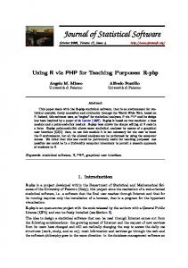
4.2. Speed comparison In order to assess the relative speed of the four packages examined, we have conducted a few experiments. In all of them we have estimated parameters in Gaussian models of different sizes by maximum likelihood. This requires repeated runs of the Kalman filter and has been done either using a function provided in the package (e.g., dlmMLE in package dlm) or writing a small function which computes the log likelihood (using the Kalman filtering routine in each package) and then handing over that likelihood to function optim for optimization. The following data sets have been used in the experiments: Nile data. This is the well-known Nile data described in Durbin and Koopman (2001) and referred to earlier. It is a short (N = 100 observations) univariate time series. A local level model involving just two parameters (ση2 and σ2 , variances of the innovation and the measurement noise) has been fitted by maximum likelihood, with all four packages and with function StructTS. Exchange rates data. Data consists of N = 2465 daily observations of the exchange rate (against the US dollar, USD) of four currencies (AUD, BEF, CHF and DEM), for the period from 1988-01-04 to 1997-08-15. Their joint evolution is displayed in Figure 1 Regression artificial data. The data consists of N = 1000 artificially generated observations from the linear model yt = β1 X1 + . . . + β5 X5 + , with βi = i for i = 1, . . . , 5. The vector β can be thought of as an invariant state vector (i.e., Qt = 0). The model can be estimated by ordinary least squares and sequentially, by means of the Kalman filter. The purpose of this experiment was to check the accuracy of the algorithms in an example with Qt = 0, which might expose numerical instability when equations (6) and (8) are used. Results. The benchmarks were run on a 2GHz. Xeon machine, running Linux and R compiled for 64 bits with an optimized BLAS library (ATLAS, see Whaley et al. 2001). A machine using a non-optimized library might see different relative performances, as some of the packages rely very heavily on BLAS. We have selected algorithm L-BFGS-B, Byrd et al. (1995), as coded in function optim in R. The feasible region for parameters (non-negative half line for variances, (−1, 1) for correlation coefficients) has been specified in the call to optim. When coding bounds for variances or correlation coefficients, we found that we had to force parameters to be slightly away from the boundary of the feasible region: lower bounds of 10−6 were given for variances and a feasible interval of (−0.99, 0.99) for correlation coefficients. Common initial values, tolerance and scaling have been used for each experiment with all four packages. The list of models fitted and the times taken are summarized in Table 2, which we comment briefly next. In the case of the Nile example (local level model fitted to a short univariate series), the interpreted nature of the sspir is seen taxing its performance very heavily: it takes much longer than the second slowest package. Even among the packages implementing the Kalman filter in compiled code, there are noticeable differences, FKF being clearly the fastest. Interestingly,

Journal of Statistical Software

17

1.2 1.4 1.6 1.8

CHF

35

40

BEF

30

Units per US dollar

1.4 1.6 1.8 2.0

DEM

0.7

0.8

0.9

AUD

1988

1990

1992

1994

1996

1998

Date

Figure 1: Daily exchange rate against the US dollar (USD) of the Australian dollar (AUD), Belgian franc (BEF), Swiss franc (CHF) and German mark (DEM). Period 1988-01-04 to 1997-08-15. in spite of using a type of square root algorithm (SVD factorization), dlm ends up being about as fast as KFAS in this particular example. The Nile example is a particular case of structural model, which can be fit most conveniently using function StrucTS. Calling, R> fit