Kernel Combination for SVM Speaker Verification R´eda Dehak1 , Najim Dehak2,3 , Patrick Kenny2 , Pierre Dumouchel 2,3 1
Laboratoire de Recherche et de D´eveloppement de l’EPITA (LRDE), Paris, France 2 Centre de recherche informatique de Montr´eal (CRIM), Montr´eal, Canada 3´ Ecole de Technologie Sup´erieure (ETS), Montr´eal, Canada
[email protected], {najim.dehak,patrick.kenny,pierre.dumouchel}@crim.ca
Abstract We present a new approach for constructing the kernels used to build support vector machines for speaker verification. The idea is to construct new kernels by taking linear combination of many kernels such as the GLDS and GMM supervector kernels. In this new kernel combination, The combination weights are speaker dependent rather than universal weights on score level fusion and there is no need for extra-data to estimate them. An experiment on the NIST 2006 speaker recognition evaluation dataset (all trial) was done using three different kernel functions (GLDS kernel, linear and Gaussian GMM supervector kernels). We compared our kernel combination to the optimal linear score fusion obtained using logistic regression. This optimal score fusion was trained on the same test data. We had an equal error rate of ≃ 5, 9% using the kernel combination technique which is better to the optimal score fusion system (≃ 6, 0%).
1. Introduction In current speaker verification systems, the best results are invariably obtained by fusing the scores of simpler subsystems. Techniques for score fusion include naive Bayes [1], Neural Network (NN) [1], Support Vector Machines (SVM) [2] and, logistic regression [3, 4]. A problem with all of these techniques (except for naive Bayes) is that held-out data is needed to properly weight the contributions of the individual subsystems. It is well known that the performance of the system can degrade drastically if there is a mismatch between the held-out data which serves to estimate the fusion weights and the data on which the system is tested. Another weakness of score-level fusion is that it is based on a single set of fusion weights, common to all target speakers. Clearly it would be desirable to allow the fusion weights to vary from one speaker to another if speakerdependent fusion weights could be reliably estimated. Speaker verification systems based on support vector machines lend themselves to another type of ‘fusion’, namely combination at the kernel level, which does not suffer from either of these drawbacks. Given a set of kernels, we can construct a new kernel for each target speaker by taking a linear combination of these kernels. There is no difficulty in principle in making the coefficients in this linear combination speaker-dependent. In fact, the coefficients can be estimated for each target speaker using the same set of imposters as serve to estimate the speakerdependent hyperplane separator in SVM training. This also dispenses with the need for held-out data to estimate score-level fusion weights. The paper is organized as follows: Section 2 presents score fusion methods. Section 3 presents the principal aspect of SVM methods. We describe the approach of kernel combin-
ing method in section 4. The kernel functions used in our experimentation are presented in 5 and the application of kernel combining in speaker verification task in 6. Section 7 presents our experiments on NIST-SRE 2006 database. We conclude the paper in section 9.
2. Score Fusion Methods The objective of score fusion method is to fuse multiple subsystems into a single effective system. By score fusion, we mean that the resulting output score of the fused system is obtained from the scores of the subsystems. Many approaches have been used to deduce the resulting score. In [5], the authors used a perceptron classifier, the fusion classifier is trained to minimize the DCF. Kajarekar [6] used a linear combination with equal weight of the scores of four different SVM systems. The most popular approach used during the last NIST Speaker Recognition Evaluation (SRE)1 campaign was the linear score fusion with a logistic regression training method [4]. The resulting score of linear score fusion is computed as: sf (x) = w0 +
M X
wi si (x)
(1)
i=1
where sf (x) is the fused output score for x test, w = (w0 , w1 , ..., wM )t a real vector of weights, si (x) is the ith subsystem score for test x and M is the number of systems which are fused. The weights vector is obtained by logistic regression training on a dataset of supervised scores.
3. Support Vector Machines An SVM [7] is a two-class classifier based on a hyperplane separators. It works by embedding the data into a Hilbert space(feature space), and searching a linear separator in this space. Usually, the feature space F has high dimensionality (potentially infinite), and is non linearly related with a mapping function φ to the original input space X . The mapping is performed implicitly, by specifying the inner product between each pair of points (x1 , x2 ) rather than giving their coordinates φ(x1 ), φ(x2 ) in the feature space explicitly. Given an observation x ∈ X and a mapping function φ, an SVM discriminant function is given by: f (x) = < w , φ(x) > + b
(2)
(w, b) are the linear separator parameters. Exploiting the kernel function and the fact that the weight vector w can be expressed as a linear combination of the training points (w = 1 http://www.nist.gov/speech/tests/spk/2006/
M P
yi αi φ(xi )), the discriminant function f can be expressed
i=1
as:
f (x) =
M X
αi yi K(xi , x) + b
This problem has been addressed in [8] and consists in finding the parameter λi that maximize the optimal margin (minimize ωC (K)).
(3)
min
The optimal linear separator is chosen in order to maximize the margin (γ = 1/kwk) defined by the distance between the hyperplane and the closest training vectors xi called support vectors (xi , i = 1...M in equation 3). The optimal parameters (w∗ , b∗ ) of this optimal separator are the solution of the primal optimization problem: < w, w >
w,b
(4)
yi (hw, φ (xi )i + b) ≥ 1, i = 1, ..., n
subject to
where yi = ±1 corresponds to xi class. Transforming this optimization problem to its dual form, the optimal squared inverse margin ω(K) = 1/γ 2 corresponding to the kernel matrix K can be expressed as follows: ω(K)
= =
< w∗ , w∗ > ` ´ max 2αt 1 − αt G(K)α
(5)
α
α ≥ 0, αt y = 0
Here G(K) = diag(y) K diag(y), K is the n × n kernel matrix of the n training points (Kij = k(xi , xj )), 1 is the n dimensional vector of ones and α is the dual variables (α ∈ Rn ). In the case of non linearly separable data, we introduce slack variables to allow the margin constraints to be violated. The primal optimization problem (4) becomes: min
< w, w > + C
w,b
n X
ξi2
(6)
i=1
yi (hw, φ (xi )i + b) ≥ 1 − ξi , i = 1, ..., n ξi ≥ 0, i = 1, ..., n
subject to
again by considering dual problem, the optimal solution of this problem can be expressed as: ωC (K)
=
< w∗ , w∗ > + C
n X
ξi2∗
(7)
i=1
=
« „ 1 max 2αt 1 − αt G(K)α − αt α α C α ≥ 0, αt y = 0
4. Combining Kernel Matrix The most important step in SVM classification systems is to define the appropriate kernel function. This function is necessary to built the kernel matrix used in the optimization problem and decision step (equation 7 and 3). Many kernel functions was proposed for speaker verification tasks. We propose here to use a linear weighted combination of these kernel matrices {K1 , ..., KN } to build a new kernel matrix K: K=
N X i=1
λi Ki
(8)
(9)
trace(K) = c
subject to:
K represents all possible kernel matrices represented by symmetric positive definite matrices. In the case of (λi ≥ 0, i = 1..N ), the optimization problem can be expressed as: max α,t
min
ωC (K)
K∈K
i=1
subject to:
1 t α α − ct (10) C 1 αt G(Ki )α, i = 1, ..., N t≥ trace(Ki ) 2αt 1 −
αt y = 0 α≥0 The optimal weight λi represents the dual variable corresponding to the ith constraint in the optimization problem. If we don’t place the λi ≥ 0, i = 1..N condition, we need to use test data to obtain the optimal weight that keep the kernel matrix positive definite (refer to [8] for more details). This procedure is not conform with NIST protocol, so we didn’t explore this solution, and we were limited to the case of λi ≥ 0, i = 1..N .
5. SVM for Speaker Verification Kernel functions used in speaker verification systems can be divided into two groups. The first one consists in applying SVMs directly to the acoustic data. This kernel defines an inner product between the mapping of two sequences in an appropriate feature space. For example, the Generalized Linear Discriminate Sequence (GLDS) kernel [9] is based on an explicit mapping of each sequence to a single vector in a feature space using polynomial expansions. Another approach implemented in [10] trains SVMs directly on the acoustics vectors which characterize the client data and the impostors data. During testing, the segment score is obtained by averaging the scores of the SVM output for each frame. Another approach proposed in [11] uses the scores obtained by the GMMs as feature vectors for the SVM classifier. The second class represents methods which use SVM in the GMMs means supervector space. The MAP adaptation can be seen as a mapping of the variable length sequence of acoustic features onto a fixed vector length. All Gaussian means vectors are pooled together to get one GMM supervector. These GMMSVM kernel functions are derived from Kullback-Leibler distance. it was proposed first in [12], and was applied for speaker verification in [13, 14] to find a separator between the speaker models and impostor models. In our experience, we have used three different kernel functions, the first one corresponds to the GLDS kernel proposed by Campbell [9]. The last ones are the linear and non linear GMM-SVM kernels. 5.1. Generalized linear discriminant sequence kernels This kernel function was proposed in [9]. Given a sequence of cepstral features xl = (x1 , x2 , ...xl ), the mapping function φglds is expressed as: φglds
:
xl −→
l 1X b(xi ) l i=1
(11)
Here b(xi ) is the vector of polynomial basis terms of feature vector xi , e.g., for two features xi = [xi1 xi2 ]t and second order, the vector is given by: ˆ ˜t b(xi ) = 1 xi1 xi2 x2i1 xi1 xi2 x2i2 (12) The GLDS kernel function kglds is defined by:
kglds (sa , sb ) = φglds (sa )t R−1 φglds (sb )
(13)
t
where R = M M and M is defined as : 2 b(xs1 )t 6 b(xs2 )t 6 ... 6 6 6 b(xsN spk ) M =6 t 6 b(xz1 ) 6 t 6 b(xz2 ) 4 ... b(xzN imp )t
3 (14)
5.2. GMM-SVM Linear kernel The linear kernel was proposed by Campbell et. al. [13]. The authors used an upper bound D of kullback-Leiber distance [15, 16] between two GMMs to built the corresponding inner product which is the kernel function as follows:
Klin (sa , sb )
=
M X
=
M „ X √
i=1
“ ” “ ”t wi µai − µbi Σ−1 µai − µbi (15) i −1 wi Σi 2 µai
i=1
wi , µsi
«„ √
7.1. Test database We performed our experiments on the core condition of NIST 2006 SRE corpus (all trials)2 . The train and test utterances contain 2.5 minutes of speech on average. The whole speaker detection task consists of 53966 tests (3612 target tests). We use equal error rate (EER) and the minimum decision cost value (minDCF) as metrics for performance evaluation. 7.2. Cepstral features
7 7 7 7 7 7 7 7 7 5
where b(xsi ) and b(xzi ) represent respectively the expansion of speaker and impostor data (see [9] for more details).
D2 (sa , sb )
7. Experiments
−1 wi Σi 2 µbi
«t (16)
Σsi
where and are the weight, mean and covariance of each Gaussian in the s speaker GMM model.
The non linear kernel is a Gaussian kernel defined on the GMMs supervector space. It was proposed by Dehak and Chollet in [14]. The kernel function is expressed as an exponential function of distance D (equation 15): Knonlin (sa , sb ) = e
7.3. SVM systems We used three SVM kernel functions in our combination. The first one is the GLDS kernel. It was constructed using the 33dimensional vector with a 3rd degree polynomial. As in [9], the R matrix (equation 13) was approximated by using only diagonal elements to reduce the training time. The two last GMM-SVM systems used in our combination are the optimal linear and non-linear kernel obtained in [17]. In these two last systems, we have used Nuisance Attribute Projection to reduce the impact of channel and handset variations on system performances (See [17] for more details). All SVM systems used single positive example and the same training impostors. A corpus of 449 male and 486 female impostors extracted from NIST-SRE 2004 and Fisher databases are used to train the SVM systems. Kernel matrices are centered and normalized as follows [7]: Centering : Kij
5.3. GMM-SVM Non Linear kernel
−D 2 (sa ,sb )
We extracted 16-dimensional Linear Frequency Cepstral Coefficients (LFCC) from speech signal every 10ms using a 20ms Hamming window. First order deltas and delta-energy are appended to the cepstral vector. Cepstral mean substraction and variance normalization were then applied to each feature of the 33-dimensional final vector.
(17)
6. Combining Kernel In Speaker Verification The weight vector of linear kernel combination is computed during target speaker models training. For each kernel function, the Gram matrix was computed using the same impostors list. The solution of the optimization problem (equation 10) provides, for each target speaker s, an optimal weight vector (λsi , i = 1..M ) and the SVM (α, b) parameters. This operation is different from score fusion methods: We have a different weight vector for each target speaker model rather than the unique score weights vector for score fusion. The most important advantages is that we don’t need extra dataset to compute the weight vector, it was computed using only training dataset. This kernel combination can be seen as an adaptation of the kernel function to the speaker data. During the training task, we change the kernel function (by selecting the weight vector λ) for each speaker and find the optimal one which gives the maximal margin.
←
Kij + −
Normalization : Kij
←
n 1 X Kmo 2 n m,o=1
n 1 X (Kim + Kjm ) (18) n m=1
Kij p Kii Kjj
(19)
To compare our results with linear score fusion approaches, we have performed two different fusions: The first one consist on naive Bayes fusion approach, all subsystems scores had 1 , i = 1..M ). The second one is the equal weight (wi = M optimal linear score fusion. In this case, the weight vector is optimized using a logistic regression [3, 4] on test data (thanks to Brummer’s FOCAL toolkits3 ). In this case, we obtain the optimal DET-curve of the fused system. This is not the natural way to implement score fusion, but we don’t have subsystems score for another database for fusion training step. These two fusion systems can be seen as the lower and the upper bound for the performances of a linear weighted score fusion system.
8. Results and Discussion We start by giving the results obtained with the three SVM subsystems using the three kernels (GLDS kernel, linear and Gaus2 See http://www.nist.gov/speech/tests/spk/ 2006/ for more details 3 See http://www.dsp.sun.ac.za/ nbrummer/focal ˜
sian GMM supervector kernels). The Table 1 gives the EER and MinDCF of these subsystems. The results show that both GMM supervector kernels perfome better than GLDS kernels. These results can be explained by the fact that we apply channel compensation algorithm (NAP) for the GMM supervector kernel SVM systems.
Speaker Detection Performance 20
Table 1: The original subsystem performance. NIST 2006 SRE core condition (all trials). System GLDS kernel Linear kernel Non linear kernel
EER 9,77% 6,75% 6,39%
MinDcf 0,045 0,032 0,030
We have tested the influence of the parameter c of the (trace(K) equation 9) on kernel combination system performance (Table 2). We note the best performances are obtained when c = 2. There is no way to fix this parameter in advance. We take this optimal value for next experiments.
Table 2: The influence of the c parameter on kernel combining system performances. NIST 2006 SRE core condition (all trials). c 0.5 1 2 5
EER 6,24% 6,17% 5,92% 6,18%
MinDcf 0,032 0,030 0,030 0,031
In Table 3, we present the performances of fusion systems. As expected, the performances of naive Bayes linear score fusion system are less than the optimal linear score fusion. This optimal version had a little improvement (0, 39% absolute) in EER. This performances are explained by the fact that all our systems used the same feature parameters with different kernel functions, we can obtain more improvements with different features. The EER obtained using the kernel combination system is better than the naive and optimal linear score fusion systems. For MinDCF performance’s, the kernel combination system is better than the naive fusion and less than the optimal linear score fusion. This performances can be explained by the fact that the kernel combination system uses a statistical criteria of maximal margin in the SVM modeling and had no prior information about the DCF function.
Table 3: Comparison between linear score fusion and linear kernel combining. NIST 2006 SRE core condition (all trials). System Naive Bayes score fusion Optimal linear score fusion Combined kernels
EER 6,28% 6,00% 5,93%
MinDcf 0,031 0,029 0,030
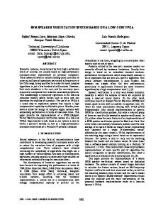
We plot on Figure 1 the DET-curves of all systems, the kernel combination system DET-curve are better than the three SVM systems and naive Bayes score fusion.
Miss probability (in %)
10
5
2
1
GLDS kernel Linear kernel Non linear kernel Naive Bayes score fusion Combined kernels Optimal score fusion 1
2
5 False Alarm probability (in %)
10
20
Figure 1: DET curve of combined kernel system, naive Bayes and optimal linear score fusion. NIST 2006 core condition (all trial)
9. Conclusions and Perspectives In this paper, we present a new method to combine SVM speaker verification systems. This method perform a fusion in kernel function space to obtain a new SVM kernel system and we don’t require extra dataset to learn the combination weights. This is an interesting advantage especially when there is a mismatch between fusion training dataset and test data. We had better performance in EER with this new technique than the optimal linear score fusion which need a development data to estimate the fusion weight parameters. We have done experiments on three different kernel functions, obtained on the same features. We plan to use this approach with more SVM systems and with different features.
10. References [1] W.M. Campbell, D.A. Reynolds, and J.P. Campbell, “Fusing Discriminative and Generative Methods for Speaker Recognition: Experiments on Switchboard and NFI/TNO Field Data,” in Speaker Odyssey, Toledo, Spain, June 2004, pp. 41–44. [2] A. Stolcke, E. Shriberg, L. Ferrer, S. Kajarekar, K. Sonmez, and G. Tur, “Speech Recognition as Feature Extraction for Speaker Recognition,” in Workshop on Signal Processing Applications for Public Security and Forensics, Washington, D.C., 2007, pp. 39–43. [3] P. Matejka, L. Burget, P. Schwarz, O. Glembek, M. Karaflat, F. Grezl, J. Cernocky, D.A. van leeuwen, N. Brummer, and A. Strasheim, “STBU System for the NIST 2006 Speaker Recognition Evaluation,” in ICASSP, Hawaii, USA, 2007. [4] Niko Brummer, Lukas Burget, Jan Honza Cernocky, Ondrej Glembek, Frantisek Grezl, Martin Karaat, David A. van Leeuwen, Pavel Matejka, Petr Schwarz, and Albert Strasheim, “Fusion of Heterogeneous Speaker Recognition Systems in the STBU Submission for the NIST
Speaker Recognition Evaluation 2006,” to appear in IEEE Trans. On Audio, Speech and Language Processing, 2007. [5] W. M. Campbell, D. E. Sturim, W. Shen, D. A. Reynolds, and J. Navratil, “The MIT-LL/IBM 2006 Speaker Recognition System: High-Performance Reduced-Complexity Recognition,” in ICASSP, Hawaii, USA, 2007. [6] S. S. Kajarekar, “Four Weightings and a Fusion: A Cepstral-SVM System for Speaker Recognition,” in Proc. IEEE Speech Recognition and Understanding Workshop, San Juan, Puerto Rico, 2005, pp. 17–22. [7] John Shawe-Taylor and Nello Cristianini, Kernel Methods for Pattern Analysis, Cambrige, 2004. [8] Gert R.G. Lanckriet, Nello Cristianini, Peter Bartlett, Laurent El Ghaoui, and Michael I. Jordan, “Learning the Kernel Matrix with Semidefinite Programming,” Journal of Machine Learning Reasearch, vol. 5, pp. 27–72, 2004. [9] W. M. Campbell, “Generalized Linear Discriminant Sequence Kernels for Speaker Recognition,” in IEEEICASSP, 2002, vol. 1, pp. 161–164. [10] M. Schmidt and H. Gish, “Speaker Identification via Support Vector Machines,” in IEEE-ICASSP, 1996, pp. 105– 108. [11] Quan Le and Samy Bengio, “Client Dependent GMM-SVM Models for Speaker Verification,” in ICANN/ICONIP, Lecture Notes in Computer Science, Ed., 2003, pp. 443–451. [12] P.J. Moreno, P.P. Ho, and N. Vasconcelos, “A Generative Model Based Kernel for SVM Classification in Multimedia Applications,” in NIPS, 2003. [13] W.M. Campbell, D.E. Sturim, D.A. Reynolds, and A. Solomonoff, “SVM Based Speaker Verification using a GMM Supervector Kernel and NAP Variability Compensation,” in ICASSP, 2006, vol. 1, pp. 97–100. [14] Najim Dehak and G´erard Chollet, “Support Vector GMMs for Speaker Verification,” in IEEE Odyssey, San Juan, Puerto Rico, 2006. [15] M.N. Do, “Fast Approximation of Kullback-Leibler Distance for Dependence Trees and Hidden Markov Models,” IEEE Signal Processing Letters, pp. 115–118, 2003. [16] M. Ben and F. Bimbot, “D-MAP: a Distance-Normalized MAP Estimation of Speaker Models for Automatic Speaker Verification,” in ICASSP, 2003, vol. 2, pp. 69– 72. [17] R. Dehak, N. Dehak, P. Kenny, and P. Dumouchel, “Linear and Non Linear Kernel GMM SuperVector Machines for Speaker Verification,” in Interspeech, Antwerp, Belgium, 2007. [18] Najim Dehak, Reda Dehak, Patrick Kenny, and Pierre Dumouchel, “The Comparison Between Factor Analysis and GMM Support Vector Machines for Speaker Verification,” in Submited to Odyssey, 2008.


![[PDF] SVM-DSmT Combination for Off-Line Signature Verification](https://m.moam.info/img/260x300/pdf-svm-dsmt-combination-for-off-line-signature-ve_59d02d161723dd6d70455751.jpg)