Kernel density estimation and its application

ITM Web of Conferences 23, 00037 (2018) XLVIII Seminar of Applied Mathematics

https://doi.org/10.1051/itmconf/20182300037

Kernel density estimation and its application Stanisław Węglarczyk1,* 1

Cracow University of Technology, Institute of Water Management and Water Engineering, Warszawska 24, 31-115 Kraków, Poland

Abstract. Kernel density estimation is a technique for estimation of probability density function that is a must-have enabling the user to better analyse the studied probability distribution than when using a traditional histogram. Unlike the histogram, the kernel technique produces smooth estimate of the pdf, uses all sample points' locations and more convincingly suggest multimodality. In its two-dimensional applications, kernel estimation is even better as the 2D histogram requires additionally to define the orientation of 2D bins. Two concepts play fundamental role in kernel estimation: kernel function shape and coefficient of smoothness, of which the latter is crucial to the method. Several real-life examples, both for univariate and bivariate applications, are shown.

1 Introduction Out of all probability distribution functions, probability density function (pdf) best shows how the whole 100% probability mass is distributed over the x-axis, i.e., over the values of an X random variable. However, the oldest pdf empirical representation  a histogram  is a highly subjective structure as its shape depends on the subjective choice of the number (or widths) of class intervals (bins) to which the range of a sample is divided, and on the choice of the initial point (e.g., [1]). To this aim several formulas have been proposed of which most relate the number of intervals to the sample size only [2–3]; the other include additionally certain sample characteristics as standard deviation [4], interquartile range [5] or skewness [6]. Independently of the class selection method used, the histogram suffers from its original sin: data binning, which depraves the data of their individual location replacing their locations with a bin (interval) location. This causes the histogram shape to become discontinuous, and flat in each bin. Kernel estimation of probability density function has not these drawbacks. It produces (in in most practical applications) a smooth empirical pdf based on individual locations of all sample data. Such pdf estimate seems to better represent the "true" pdf of a continuous variable. Kernel estimation is not a quite new technique: it was originated more than a half century ago by Rosenblatt [7] and Parzen [8]. With the development of computer technology, this method has been developing rapidly and vastly [4, 9–17]. The paper shows the advantages and disadvantages of the method illustrating them with real-life examples for one- and two-dimensional applications.

*

Two concepts play fundamental role in kernel estimation: the kernel function and the coefficient of smoothness.

2 Kernel density Let the series {x1, x2,..., xn} be an independent and identically distributed (iid) sample of n observations taken from a population X with an unknown probability distribution function f(x). Kernel estimate fˆ ( x) of original f(x) assigns each i-th sample data point xi a function K(xi,t) called a kernel function in the following way [11]: 1 n fˆ (t )   K ( xi , t ) n i1

(1)

K(x,t) is nonnegative and bounded for all x and t: 0  K ( x, t )   for all real x, t

(2)

and, for all real x, 

 K ( x, t )dt  1.

(3)



Property (3) ensures the required normalization of kernel density estimate (1): 







1 fˆ (t )dt    K ( xi , t )dt  1. n i1  n

(4)

In other words, kernel transforms the "sharp" (point) location of xi into an interval centred (symmetrically or not) around xi.

Corresponding author: [email protected]

© The Authors, published by EDP Sciences. This is an open access article distributed under the terms of the Creative Commons Attribution License 4.0 (http://creativecommons.org/licenses/by/4.0/).



In most common practical applications, the kernel estimation uses symmetric kernel function, although asymmetric functions have recently been increasingly used [18–20]. Figs. 1 and 2 illustrate the idea of kernel estimation for both cases.

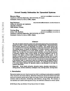
Fig. 3. The value of the smoothing parameter h influences the shape of the resulting kernel density. The 4-element sample (vertical segments) are the same as in Figs. 1 and 2.

Many types of kernel function can be found in the relevant literature. Examples of symmetric kernels are presented in Table 1 and in Fig. 4, while Table 2 shows the asymmetric ones.

Fig. 1. Construction of kernel density estimator (1) (continuous line) with a symmetric kernel (dashed lines) for a 4-element sample (vertical segments).

Table 1. Examples of symmetrical kernel functions [11]. Kernel Epanechnikov

Definition

 3 (1  15 t ) 2 for t  5 4 5

K (t )  

for t  5

 0

 1615 (1  t ) for t  1  for t  1 0 2

Biweight

Triangular

Fig. 2. Construction of kernel density estimator (1) (continuous line) with an asymmetric kernel (dashed lines) for the same 4element sample as in Fig. 1.

Fig. 1 shows that the shape of a symmetric kernel is the same for all sample points while Fig. 2 reveals that the shape of an asymmetric kernel differs with the point placement. Symmetry property allows to write the kernel function in a form used most frequently:

K sym ( x, t ) 

1  x t  K  h  h 

K (t ) 

2

 1  t for t  1 for t  1  0

K (t )  

1 t 2 / 2 e 2

Gaussian

K (t ) 

Rectangular

K (t )   2

1  for t  1 0 for t  1

Table 2. Examples of asymmetrical kernel functions. Symbol b denotes the smoothing parameter. Kernel

Definition x / b t / b

Gamma 1 [18]

K GAM 1 ( x, b; t ) 

(5)

t e b

x / b 1

( x / b  1)

KGAM 2 ( b ( x), b; t ) 

where parameter h, called smoothing parameter, window width or bandwidth, governs the amount of smoothing applied to the sample (Fig. 3). For symmetrical kernel functions, the choice of the shape of the kernel function K(.) has rather little effect on the shape of the estimator [11, 21], whereas  as Fig. 3 shows  the influence of the smoothing parameter h is critical because it determines the amount of smoothing. Too small value of h may cause the estimator to show insignificant details while too large value of h causes oversmoothing of the information contained in the sample, which, in consequence, may mask some of important characteristics, e.g. multimodality, of f(x) (cf. Fig. 3). A certain compromise is needed.

Gamma 2 [18]

Inverse Gaussian [19] Reciprocal Inverse Gaussian [19] Lognormal [20]

2

t b ( x ) 1et / b b ( b ( x)) b ( x )

for x  2b x / b b ( x )   1 2  4 ( x / b)  1 for x  [0,2b) K IG ( x, b; t ) 



1 2 bt

3

e

1 t x  2  2 bx  x t

x b  t

K RIG ( x, b, t )  K LN ( x, b; t ) 

  2  1 e 2b  x  b 2 bt

1 8 ln(1  b)t



e

x b   t 

 ln t  ln x 2 8 ln(1 b )



Two versions of (6) are used in practice: the product kernel estimator and the radial kernel estimator [24]. In its most popular form, the product kernel estimator may be written as follows

fˆ ( x, y ) 

1 nhx hy

 xi  x   y j  y    K   hx   hy 

n

K  i 1

(7)

The radial kernel estimator is based on the Euclidean distance between an arbitrary point {x,y} and sample point {xi,yi}, i = 1,2, ..., n:

Fig. 4. Shapes of symmetric kernels defined in Table 1.

Fig. 5 illustrates how the kernel type (cf. Table 1) used to estimate pdf influences the kernel pdf estimate. Triangular and rectangular kernels (especially the latter) produce many local maxima and thus they are rather not recommended for application. The biweight kernel has shorter support than the Epanechnikov one, so reveals more details and more clearly suggests two basic modes. The Gaussian kernel, distributed over the whole x-axis, produces the most smooth estimate, and this property probably causes the kernel to be most frequently used.

fˆ ( x, y ) 

1 nhx hy

  x  x 2  y  y 2 i   i K    h   h i 1   x   y  n

  (8)  

In practice, the product kernel estimator is mostly used. The advantage of multivariate kernel pdf over multivariate histogram is even greater than in an univariate case. This is because of an additional subjective requirement occurs: the user has to decide about the orientation of a two-dimensional bin, which may considerably influence the final shape of the histogram.

3 Measures of discrepancy between the kernel density estimator fˆ and the true density f Each estimator fˆ ( x) differs from its original f(x) with 100% probability. In order to build a method producing an estimator fˆ ( x) which will be as close to f(x) as possible, certain measures should be defined to evaluate this discrepancy. For each single x, a difference between the "true" density function f(x) and its estimator fˆ ( x) can be estimated with the mean squared error, MSEx, [11]:

 

Fig. 5. Different symmetrical kernel functions applied to a sample of 45 standardized annual maximum flows (1961–1995) of Odra river recorded at the Racibórz-Miedonia gauge station (data source: [22]).

1 nhx hy

n

 xi  x y j  y  ,  hy   hx

 K  i 1



(9)

which, after simple transformations, can be presented as follows:

The univariate case can be easily formally extended to the multivariate case [23]. However, its illustrative (graphical) power works well for bivariate case only. The most frequently used bivariate kernel function is symmetric

fˆ ( x, y) 



2 MSE x fˆ  E  fˆ  x   f  x    

  



MSE x fˆ  Efˆ  x   f  x   var fˆ  x  2

  bias fˆ  x    var fˆ  x    2

(10)

that is, MSEx is the sum of the square bias and the variance of fˆ ( x) at x. Reducing the bias causes variance to increase and vice versa, so a trade-off between these terms is needed. MSEx is a local measure. Integration of MSEx over all x gives a global measure of conformity of fˆ ( x) with f(x), called the mean integrated square error, MISE, [11]:

(6)

where {xi, yi}, i = 1,2,...,n, is a sample, and hx and hy are smoothing coefficients. Available are multivariate counterparts of univariate kernel functions listed in Table 1, e.g., multivariate Epanechnikov kernel or multivariate Gaussian kernel [11].

3



 

 MISE(fˆ )   MSE x fˆ dx -

     bias fˆ  x   dx   var fˆ  x  dx  -  - 2

The value (15) is widely used in practice and referred to as the Silverman’s bandwidth or (Silverman’s) rule of thumb, and will be used in most of the remainder of the paper.

(11)

MISE is one of measures used to estimate the smoothing parameter. In practice, an approximate version of MISE, called AMISE (asymptotic MISE) is also used, developed by expanding MISE into a Taylor series and taking only the most important parts [25, 26]. Integrated square error, ISE, is an intermediate measure, between MISE and MSE:

ISE(fˆ ) 



  fˆ  x   f  x  dx

4.2 Least squares cross validation method (LSCV) The least squares cross validation method (LSCV) of selecting the smoothing parameter is a very popular technique [11, 30, 33–38]. LSCV uses the integrated square error, ISE (12), which can be expressed in the following form 11: 

2

(12)

ISE (h) 



  fˆ  x   f  x  

2

dx





which is also a discrepancy measure used to estimate the magnitude of the smoothing parameter.









fˆ 2  x dx  2  fˆ  x   f  x  dx

(16)





  f 2  x dx

4 Methods for calculating optimum value of smoothing parameter



The last part of the expression (16) does not depend on the estimator fˆ ( x) (it is a constant), therefore the choice of the smoothing parameter (in the sense of minimizing ISE) will correspond to the choice of h which minimizes the function

The choice of the optimal smoothing parameter is based, i.a., on formulas that minimize the criterion functions discussed above, mainly ISE [27], MISE [28] and AMISE [11, 15, 29–32]. Many other methods for calculating the smoothing parameter are available in the relevant literature; many of them are available also through statistical software. Two methods are described below  one for the symmetrical kernel function (Gaussian), the other for any kernel function.

(17)



1 fˆi  x    K  x, x j  n  1 j i

(18)

which is an estimate of the density function calculated using all sample values except xi. The resulting form of the LSCV criterion function is

(13)

LSCV  h  

where ˆ is the sample standard deviation and n is the sample size. In order to have an estimator more robust against







2 fˆ 2  x  dx   fˆi  xi  n i

(19)

The optimal smoothing parameter hLSCV is the value for which the LSCV(h) function achieves the minimum. The final form of LSCV function (19), applicable to both symmetrical and asymmetrical kernels, is:

outliers the sample interquartile range IRQ may be applied [11]: (14)

LSCV  h  

Silverman [11] believes that the value (13) smoothes non-unimodal distributions too much, and  as one of the remedies  proposes a slightly reduced value of the smoothing parameter (13):

 IQR  1/5 h  0.9  min  ˆ , n  1.34   

 x  dx  2  fˆ  x   f  x  dx

To estimate the second part of (17) a leave-one-out density estimator, fˆi  x  , is used:

The rule-of-thumb method is based on the asymptotic mean integrated square error, AMISE, when the kernel function and true distribution are assumed normal. Silverman [11] got then the values of the smoothing parameter h as follows:

h  0.79  IQR  n1/5



2



4.1 Rule-of-thumb method

h  1.06  ˆ  n1/5



   fˆ

R fˆ 

1 n2



  K  x, x  K  x, x dx i

i , j 

2   K  xi , x j  n(n  1) i j  i

j

(20)

Least squares cross-validation is also referred to as unbiased cross-validation 26. Unfortunately, the LSCV method also has drawbacks: the variance of the obtained smoothing

(15)

4



parameters calculated for samples drawn from the same distribution is large [30]. It happens that the LSCV(h) function has several minimums, often false and far on the side of too small smoothing [39]; sometimes LSCV(h) does not have any minima at all [14, 30]. There are other versions of the cross-validation method, e.g. biased cross-validation (BCV) or smoothed cross-validation (SCV), and other methods to obtain optimum smoothing coefficient (e.g., [40]). Some resulting examples are shown in Fig. 6.

Fig. 7. Kernel density estimates for four 45-year time series of standardized annual maximum flows (1961–1995) of given River/Gauging station (data source: [22]).

Fig. 8. Kernel density estimates for four 32-year time series of standardized annual minimum flows (1983–2015) of given River/Gauging station (data source: [41]).

Fig. 6. Different methods for kernel smoothing coefficient estimation available in Wolfram Mathematica 11.1 applied to the 1961–1995 series of standardized annual maximum flows of Odra river recorded at the Racibórz-Miedonia gauge station (data source: [22]).

5 Kernel density in practice 5.1 The univariate case Figs. 7 through 9 contain several kernel pdf estimates obtained for maximum and minimum annual flows of certain rivers and maximum annual precipitations in Poland. Apart from the nice smoothness contrasting with a histogram shape, a very attractive characteristic of kernel estimation is shown: its ability to suggest multimodality in a more convincing way than the histogram does.

Fig. 9. Kernel density estimates for four 30-year time series of standardized annual maximum precipitation (1984– 2013) at given Precipitation station/River basin/ (data source: [42]).

Of course, the multimodal shape of a pdf estimate does not prove the existence of the real multimodality. It is, however, a sign of possible non-homogeneity that should be considered through the analysis of the mechanism generating the data. Some attempts to statistical testing multimodality are described in [11];

5



however, as Silverman ([11], p. 141) conclude: "It may be futile to expect very high power from procedures aimed at such broad hypotheses as unimodality and multimodality". Nevertheless, the kernel estimation is a good method for an initial stage of the planned study on probability distribution. When the variable under study is nonnegative, it may happen that kernel estimate exhibits an undesirable case: probability leakage below zero. It occurs when a part of the sample lies near zero and the magnitude of the smoothing coefficient enables such crossing in a considerable amount. Four such cases are presented in Fig. 10.

If the amount of the probability leakage cannot be disregarded, one of the remedies is to logarithmize the data and apply the kernel estimation to such data. If pdf of logarithmized data is gˆ( x) the following recalculation should be used: 1 fˆ ( x)  gˆ (ln( x)) x

(21)

Fig. 11(b) shows the result. The leakage has been removed; unfortunately, the second mode disappeared although certain suggestion of non-unimodality has remained visible in the heaviness of the right tail. Another remedy is to use an asymmetric kernel shown in Fig. 11(c). This approach shows the bimodality revealed in Fig. 11(a). In terms of cumulative distribution function (Fig. 11(d)), log transformation and asymmetric kernel approach are almost equivalent. 5.2 The bivariate case and some general remarks on the multivariate case Formally, the univariate case can be easily extended to the multivariate one, which has been exemplified by equations (7) and (8) for the bivariate kernel. Fig. 12 illustrates with the use of equation (7) how the relation between the two variables studied evolves over the year. 2D kernel pdf graphics may help the user in differentiating the sample into subsamples, for which a non-statistical (cause-and-effect) confirmation may be found. Such graphics is informative when a sample contains many identical data, which are not visible in an x-y plot. Unfortunately, graphical illustration or interpretation for more than two-variate case is at least difficult if not impossible. Moreover, sample size necessary for preserving similar accuracy as that for one-dimensional case grows rapidly with growing dimension  the problem known as the 'curse of dimensionality'. Minimization of the effect of the curse of dimensionality requires not only sufficient data, but also careful data preparation [23]. This may involve proper transformation of marginal variable in order to reduce the large skewness or heavy tails, determination if the data are of full rank, and even  if the data do not have many significant digits  carefully blurring the data [23].

Fig. 10. Probability leakage below zero (marked dark blue) in kernel density estimates for time series of standardized annual maximum flow (1961–1995), top two graphs, and annual minimum flows (1983–2015), bottom two graphs, of given River/Gauging station (data source: [22]). The numbers within the graphs show the magnitude of probability leakage.

6 Summary and conclusions When compared with the commonly used histogram, the kernel density estimator shows several advantages. 1. It is a smooth curve and thus it better exhibits the details of the pdf, suggesting in some cases nonunimodality. 2. It uses all sample points' locations, so, therefore, it better reveal the information contained in the sample. 3. It more convincingly suggests multimodality. 4. The bias of the kernel estimator is of one order better than that of a histogram estimator [26]. 5. Compared with 1D application, 2D kernel applications are even more better as the 2D histogram

Fig. 11. Removing probability leakage below zero (4.9%, marked dark blue) in kernel density estimate (a) of the 1984– 2015 time series of standardized annual maximum flows ; (b) logarithmized pdf added; (c) asymmetric gamma kernel pdf added (cf. Table 2, kernel KGAM1, b = 0.06); (d) three cumulative distribution functions (data source: [41]).

6



requires additionally the specification of the orientation of the bins which enhances the subjectivity of histogram. It should be remembered, however, that the value of smoothing coefficient is to some extent a subjective estimate.

References 1. S. Węglarczyk., M. Kulig, Wiad. IMGW XIV(XLV), Z.2, 59–69 (2001) 2. H.A. Sturges, J. Amer. Statist. Assoc. 21, 65–66 (1926) 3. C. E. P. Brooks, N. Carruthers, Handbook of statistical methods in meteorology (HM Stationary Ofﬁce, London, 1953) 4. D.W. Scott, Biometrica 66, 605–610 (1979) 5. D. Freedman, P. Diaconis, Zeit. Wahr. ver. Geb. 57(4), 453–476 (1981) 6. D. P. Doane, American Statistician 30(4), 181–183 (1976) 7. M. Rosenblatt, Annals of Mathematical Statistics 27, 832–837 (1956) 8. E. Parzen, Annals of Mathematical Statistics 33, 1065–1076 (1962) 9. A. Bowman, Journal of Stat. Comp. Simul. 21, 313– 327 (1985) 10. G.R. Terrel, D.W. Scott, Journal of the American Statistical Association 80(389), 209–214 (1985) 11. B.W. Silverman, Density estimation for statistics and data analysis (Chapman and Hall, London, 1986) 12. L. Devroye, Annales de l’Institut Henri Poincaré 25, 533–580 (1989) 13. G.R. Terrel, Journal of the American Statistical Association 85, 470–477 (1990) 14. S.J. Sheather, Computational Statistics 7, 225–250 (1992) 15. J.S. Marron, M. P. Wand, Annals of Statistics 20, 712–736 (1992) 16. L. Devroye, Statistics and Probability Letters 20, 183–188 (1994) 17. L. Devroye, A. Krzyżak, Journal of Multivariate Analysis 82, 88–110 (2002) 18. S.X. Chen, Annals Of The Institute of Statistical Mathematics 52(3), 471–480 (2000) 19. O. Scaillet, Density estimation using inverse and reciprocal inverse gaussian kernels (IRES Discussion Paper 17, Université Catolique de Louvain, 2001) 20. X. Jin, J. Kawczak, Annals of Economics and Finance 4, 103–124 (2003) 21. P. Hall, J.S. Marron, The Annals of Statistics 15(1), 163–181 (1987) 22. B. Fal, E. Bogdanowicz, W. Czernuszenko, I. Dobrzyńska, A. Koczyńska, Przepływy charakterystyczne głównych rzek polskich w latach 1951–1995 (in Polish: Characteristics flows of main rivers in Poland in 1951–1995) (Materiały Badawcze, Seria: Hydrologia i Oceanologia 26, Instytut Meteorologii i Gospodarki Wodnej, Warszawa, 2000)

Fig. 12. Bivariate kernel density estimates for two-dimensional random variable (monthly maximum temperature tmx, and monthly sunshine duration, S), in Oxford, UK, 1853–2017 (data source:[43]).

7



23. D. W. Scott, Multivariate Density Estimation, Theory, Practice, and Visualization (John Wiley and Sons, Inc., 1992) 24. W. Härdle, M. Müller, S. Sperlich, A. Werwatz, Nonparametric and Semiparametric Models (Springer, 2004) 25. T. Ledl, Austrian Journal of Statistics 33(3), 267–279 (2004) 26. S.J. Sheather, Statist. Sci. 19(4), 588–597 (2004) 27. S.R Sain, Adaptive kernel density estimation, (PhD diss., Rice University, http://hdl.handle.net/1911/ 16743, 1994, accessed June 2018) 28. J.S. Marron, D. Nolan, Statistics and Probability Letters 7, 195–199 (1989) 29. A. Bowman, P. Hall, T. Prvan, Biometrika 85(4), 799–808 (1998) 30. B.A. Turlach, Bandwidth selection in kernel density estimation: A Review (Discussion Paper, C.O.R.E. and Institut de Statistique, Université Catolique de Louvain-la-Neuve, Belgium, 1993) 31. W. Feluch, Wybrane metody jądrowej estymacji funkcji gęstości prawdopodobieństwa i regresji w hydrologii (in Polish: Selected methods for kernel estimation of probability density function and regression in hydrology) (Prace Naukowe Politechniki Warszawskiej 15, Oficyna Wydawnicza Politechniki Warszawskiej, Warszawa, 1994) 32. E. Choi, P. Hall, Biometrika 86(4), 941–947 (1999) 33. P. Hall, S.J. Sheather, M.C. Jones, J.S. Marron, Biometrika 78(2), 263–269 (1991) 34. S.T. Chiu, Statistica Sinica 6, 129–145 (1996) 35. S.T. Chiu, The Annals of Statistics 19(4), 1883–1905 (1991) 36. S.T. Chiu, Biometrika 79(4), 771–782 (1992) 37. M. Rudemo, Scand. Journal of Statistics 9, 65–78 (1982) 38. A. Bowman, Biometrica 71, 353–360 (1984) 39. P. Hall, J.S. Marron, Journal of the Royal Statistical Society B(53), 245–252 (1991) 40. A. Michalski, Meteorology Hydrology and Water Management 4(1), 40–46 (2016) 41. Roczniki Hydrologiczne 1984–2015, IMGW-PIB (Institute of Meteorology and Water Management National Research Institute), CD-ROM 42. IMGW-PIB (Institute of Meteorology and Water Management - National Research Institute) 43. www.metoffice.gov.uk/pub/data/weather/uk/ climate/stationdata/oxforddata.txt (accessed May 2018)

8