crucial impact in diverse domains, ranging from bioinformat- ics, medical science ... recently proposed to make it more
Kernel Methods for Minimum Entropy Encoding Stefano Melacci and Marco Gori Department of Information Engineering, University of Siena, 53100 Siena, Italy {mela,marco}@dii.unisi.it
Abstract—Following the basic principles of InformationTheoretic Learning (ITL), in this paper we propose Minimum Entropy Encoders (MEEs), a novel approach to data clustering. We consider a set of functions that project each input point onto a minimum entropy configuration (code). The encoding functions are modeled by kernel machines and the resulting code collects the cluster membership probabilities. Two regularizers are included to balance the distribution of the output features and favor smooth solutions, respectively, thus leading to an unconstrained optimization problem that can be efficiently solved by conjugate gradient or concave-convex procedures. The relationships with Maximum Margin Clustering algorithms are investigated, which show that MEEs overcomes some of the critical issues, such as the lack of a multi-class extension and the need to face problems with a large number of constraints. A massive evaluation on several benchmarks of the proposed approach shows improvements over state-of-the-art techniques, both in terms of accuracy and computational complexity.
I. I NTRODUCTION Clustering is a central topic in machine learning that has a crucial impact in diverse domains, ranging from bioinformatics, medical science, computer vision to information retrieval [1]. Clustering algorithms aim at discovering the underlying structure of the data, grouping examples into a number of classes, or clusters, such that the entities belonging to the same cluster are “similar” to each other and “different” from the ones of the other clusters. Popular examples include KMeans, Mixture Models [1], and Spectral Clustering [2]. More recently, Maximum Margin Clustering (MMC) has received an increasing interest in the scientific community [3]. MMC extends the maximum margin principle to unsupervised learning, leading to state-of-the art performances in many applications. MMC learns the optimal hyperplane that separates dense regions of points, while maximizing the margin. The learning problem behind MMC is intrinsically complicated and several relaxations of the original formulation have been recently proposed to make it more affordable. Xu et al. [3] formulate a convex semi-definite programming problem, whereas Valizadegan and Jin [4] propose Generalized Maximum Margin Clustering (GMMC) that reduces the number of variables from O(n2 ) to O(n), where n is the data set size. Zhang et al. [5] propose IterSVR, an iterative solution based on a set of support vector regression problems. Similarly, the cuttingplane based approach (CPMMC) in [6] has been proven to be an efficient method for large scale MMC. The optimization is still not-convex, with a large number of constraints, and it is solved using a cutting-plane strategy and a constrained concave-convex procedure (CCCP) [7]. Finally, in order to
preserve convexity, a tighter and convex relaxation (LGMMC) of the original MMC is proposed in [8]. Inspired by the Information-Theoretic Learning (ITL) framework [9], different algorithms for feature extraction, dimensionality reduction, and clustering have been recently studied [10]–[12]. In particular, the conditional entropy can be interpreted as a measure of class overlap [13], which is related to the quality of the data partitioning. The minimization of the conditional entropy under a smoothness assumption converges to solutions that are close to MMC [12]. In this paper, we introduce Minimum Entropy Encoders (MEEs), that are designed to learn a set of functions projecting each input point onto a minimum entropy configuration (code) of length d, where d is the number of clusters. The code collects the cluster membership probabilities, and the encoding functions are modeled by means of kernel machines. The optimization problem of MEEs consists of the sum of three terms that embed three crucial properties in the encoders: minimize the conditional entropy, ensure that the distribution of the output features is balanced, and enforce smooth solutions. There are three main contributions in this paper. First, we introduce MEEs as the solution of a minimization problem based on a suitable regularization of the entropy, and show that such a solution is given in terms of kernel machines. MEEs learn cluster separation hyperplanes in low-density regions and balance the distribution of the output features. This avoids any additional constraints [3], [4], [6], [8] or iterative label-switching mechanisms [12]. Second, we present efficient ways to solve the unconstrained MEE problem by means of conjugate gradient or CCCP. Using the former, MEE has time complexity O(n2 dT ), where T is the number of iterations, that we empirically found to be T 0 is the classic regularization parameter to enforce ˆ F ) ranges in the smoothness of the solution. Since −µH(X, [−µ log d, 0] we can eventually add the offset µ log d to ensure that (5) is nonnegative. Since we do not know in advance if the d clusters are balanced, a soft-constraining scheme with a tunable parameter µ appears an appropriate choice. When scaling the terms of (4) properly, we can easily realize that the optimal solution of the problem is independent of the log base. For the sake of simplicity, we define pij := pj (xi , F ), Pd−1 and wi := 1 + z=1 efz (xi ) . In turn, the conditional entropy H(Y |X, F ) (3) can be rewritten as n
d
1 XX pij ln (pij ) n i=1 j=1 � fj (xi ) � � � n d−1 n 1 XX e 1X 1 = − pij ln − pid ln n i=1 j=1 wi n i=1 wi
H(Y |X, F ) = −
n d−1
= −
n
1 XX 1X pij fj (xi ) + ln (wi ) . n i=1 j=1 n i=1
(6)
Interestingly, the hypothesis of looking for solutions belonging into the RKHS of k has a strong consequence in the optimization of 4. Theorem 2.1: Let f j ∈ H, where H is the RKHS of kernel k(·, ·). Then fj = arg minf ∈H C(F ) is given by j
fj (x) =
n X i=1
αij k(xi , x)
Proof: The proof can easily be given by following the classic scheme reported in [16] p. 90-91. Now, let K ∈ IRn,n be the Gram matrix associated to the points in X, kj ∈ IRn is j-column of K, and kij is the element in position (i, j). Analogously, A ∈ IRn,d−1 is the matrix of the coefficients αij , and αj ∈ IRn is its j-th column. P ∈ IRn,d collects the probabilities pij . 1n is the column vector composed of n elements equal to 1. The symbol ◦ is the element-wise product between two arrays or matrices, and ln(·) and e(·) are assumed to operate element-wise on vectorial data. We define d˜ = d − 1, and we use the notation P˜ to indicate the matrix composed with first d˜ columns of P . Finally, (5) can be written in matrix notation as � (1 − µ) T � ˜ C(A) = 1n (−P ◦ (KA))1d˜ + ln(1n + 1d˜eKA ) n� � µ 1 T T − ((−1n P ) ◦ (ln 1n P ))1d − nlnd n n +λ1Tn ((KA) ◦ A)1d˜. (7) III. T RAINING
THE
E NCODER
Training an MME consists in minimizing C(A) (7) with respect to the matrix of coefficients A. The objective function is continuous, differentiable, and it is composed of the sum of a concave part, i.e. (1 − µ)H(Y |X, F ) (bounded in [0, ln d]), ˆ F ) and λΩ(F ), so that it and two convex ones, i.e. −µH(X, is bounded below and not convex. We optimized the problem using a nonlinear Conjugate Gradient (CG) with line search performed by the secant method and Polak-Ribiere update [18], that avoids the computation of second derivatives, and it is popularly used for its speed and easy implementation. In Section III-A we will describe how to efficiently simplify the gradient expression to avoid a costly matrix-by-matrix product. Alternatively, MEEs can be trained using convex optimization tools by means of a concave-convex procedure (CCCP) [7]. CCCP allows C(A) to be minimized by iteratively solving a set of convex problems. Given At at time t = 0, we indicate with u(A) and −v(A) the convex and concave portions of C(A), so that C(A) = u(A) − v(A), and Cconvex (A, At )
= u(A) − 1Tn (A ◦ ∇v(At ))1d˜,
is a convex function obtained by linearizing the concave part of C(A) around At . Finally At+1 = arg min Cconvex (A, At ). Now we discuss two important issues of both the optimization schemes. Firstly, different starting points of the optimization, A0 , can lead to different suboptimal results. A a good choice A0 can reduce the optimization times and improve the quality of the solution. Second, when evaluating different solutions, smaller values of the objective function may not always correspond to a better data partitioning, and a criterion to select the most promising one must be devised. Beyond a random initialization of A0 , a we suggest to run a few K-Means iterations to get an initial guess of the ˜ data partitioning. We denote with Ykm ∈ {−1, 1}n,d the label matrix generated by K-Means, where the element in position
(i, j) is 1 if xi was predicted to belong to cluster j (when it belongs to cluster d, then the i-th line is composed only of −1s). If we fit the targets of Ykm with the functions f1 , . . . , fd˜, then yi = arg maxj pj (xi , F ) will match the KMeans prediction. For instance, we can solve a regularized least-square problem, leading to A0 = (K + λI)−1 Ykm [19]. We notice that each permutation of the columns of A0 will lead to equivalent solutions (the permutation will be applied to the output codes). Selecting A0 = 0·1n 1Td˜ leads to f1 , . . . , fd˜ that are equivalent and constant, and each input point is projected into the same output code [1/d, . . . , 1/d]. It is a degenerate solution of the problem, it must be avoided. Moreover, without performing any additional machinery we have the use of the conditional entropy H(Y |X, F ) associated to each solution, that is one of the three terms that compose (5). Hence, once µ and λ have been fixed, we can optimize the algorithm from different starting points and select the solution that corresponds to the smallest H(Y |X, F ). A. Gradient Computation In this section we describe how to compute the gradient ˜ matrix ∇C(A) ∈ IRn,d and how to dramatically simplify its computation avoid a product by K. ∇C(A) is the sum of three elements, ˆ F ) + λ∇Ω(F ). ∇C(A) = (1 − µ)∇H(Y |X, F ) − µ∇H(X, (8) Considering that fj (xi ) = kTi αj , we have ! n X d˜ X ∂H(Y |X, F ) ∂pij ∂kTi αj T = − · ki αj + pij · ∂αzh ∂αzh ∂αzh i=1 j=1 +
n X
pih ·
i=1
∂kTi αh . ∂αzh
(9)
The derivatives of pij and kTi αj with respect to αzh can be straightforwardly computed, and they can be expressed using the Kronecker delta δhj , ∂pij = (pij δhj − pij pih ) · kiz , ∂αzh
∂kTi αj = δhj kiz . (10) ∂αzh
Plugging them in (9), we get d˜
n
XX ∂H(Y |X, F ) = − kiz (pij kTi αj δhj − pij kTi αj pih ), ∂αzh j=1 i=1 and, switching to matrix notation,2 � � �� ∇H(Y |X, F ) = −K P˜ ◦ KA − (P˜ ◦ (KA))1d˜1Td˜ .(11)
We follow the same procedure to compute the gradient of ˆ F ). In detail, H(X, ! ! d X n n X ˆ F) ∂H(X, ∂pij 1X = − ln prj + 1 . ∂αzh ∂αzh n r=1 j=1 i=1 2 Due
to space constraints, we do not report all the derivations.
After we introduce sj = ln results of (10), we get ˆ F) ∂H(X, ∂αzh
=
−
1 n
Pn
d X n X
r=1
� prj + 1 and we use the
1.5
1
1
0.6
4
0.4
3
0.5
2
0.2 0.5
1 0
0 0
0 −0.2
−1
−0.5
(sj pij δhj − sj pij pih ) · kiz .
j=1 i=1
Finally, passing to matrix notation,2 � � ˆ F )=−K P˜ ◦ (1n (ln 1 1T P )T − P (ln 1 1T P )1T˜ ) . ∇H(X, d n n n n (12) Now we can plug (11), (12) and ∇Ω(F ) = 2KA into (8), and complete the derivation of the gradient, �� µ−1 �˜ � ∇C(A) = K P ◦ KA − (P˜ ◦ (KA))1d˜1Td˜ n � � µ 1 T 1 T T T ˜ + K P ◦ (1n (ln 1n P ) − P (ln 1n P )1d˜ ) n n n +2λKA. (13) Each stationary point of C(A) satisfies ∇C(A) = 0 · 1n 1Td˜ . This set of equations can be simplified by solving their preconditioned form ∇′ C(A) = K −1 ∇C(A) = 0 · 1n 1Td˜ , where ∇′ C(A) can be computed without performing any matrix inversions, since K is a factor of ∇C(A).3 This preconditioned form of the gradient avoids the need of a costly matrix-bymatrix product, and we can efficiently apply the CG algorithm. More details are discussed in Section III-B. Finally, the expansion of fj (x) can be augmented with a not-regularized bias bj , i.e. fj (xi ) = kTi αj + bj . The vector ˜ Following the same strategy that b collects bj , j = 1, . . . , d. we used for A, we can get that the gradient of the objective function with respect to b is simply the vector that collect the sum (column-wise) of the preconditioned gradient with respect to A, ∇′A C(A), computed with λ = 0, �T ∇bC(A) = 1Tn · ∇′A C(A) λ=0 . B. Complexity Analysis
When MEEs are trained using CG, each iteration requires to store the matrix A, ∇′ C(A), and the current descent direction, ˜ that belong to IRn,d (we discard the bias term, for simplicity). ˜ If the matrices KA ∈ IRn,d and P ∈ IRn,d are stored when evaluating the objective function (7), then the computation of the gradient ∇′ (A) can be significantly accelerated. Optionally, also the Gram matrix K ∈ IRn,n can precomputed. Hence, in the worst case, the space complexity is bounded O(n2 ) (since d ≤ n).4 CPM3C [15], the most efficient multiclass MMC algorithm, has a space complexity of O((n + d)D + ndm). D is the dimensionality of the input data in the case of linear kernels. In the nonlinear case, the authors suggest to exploit an explicit embedding with Kernel PCA [16], and D ≤ n, so that the 3 We are assuming that in this expression K is non singular, otherwise we can suppose that a small ridge is added to fix it. 4 This analysis considers a generic kernel function (linear, nonlinear), without any distinctions. However, in the linear case the complexity can be reduced, and we leave to future work this specific study.
−0.5
−1 −2
−0.4
−2
−1 −1
0
1
2
3
−1
−0.5
0
0.5
1
−0.4
−0.2
0
0.2
0.4
0.6
−3 −10
−5
0
5
10
Fig. 1. Examples of clustering results produced by MEEs (different color/markers represent data from different classes). The rightmost data set is composed of 3 Gaussian distributions in IR10 , linearly separable only on the first dimension (the first 2 ones are plotted).
worst case is O(n2 + ndm). The variable m is the average number of cutting-plane iterations, and it is problem dependent for multiclass data (theoretical results are given only in the 2-class case [15]). Moreover it depends on the degree of fulfillment of the problem constraints, that are an exponential number (i.e. (d + 1)n [15]). In Section IV, we show that this space requirements can make CPM3C impractical in some benchmarks, whereas we have been able to efficiently complete them with MEEs. ˜ ) due to the Training an MEE has time complexity O(n2 dT KA product, where T is the number of CG iterations. We experimentally evaluated that we can find a solution in just few steps, as we investigate in Section IV. Differently, from a practical point of view CPM3C scales roughly linearly with n when using a linear kernel, whereas in the nonlinear case it becomes O(n3 ) due to computational burden of the data embedding process. IV. E XPERIMENTAL R ESULTS Before discussing more detailed comparisons, the outcome of MEE-based clustering on some synthetic datasets is reported in Fig. 1, showing the capability of MEEs to correctly separate clusters in non-dense regions. We tested MEEs in several UCI data sets, in the digit recognition benchmark USPS (selecting the test portion, USPST) and in the object recognition data set Coil20. We compared MEEs with the related clustering algorithms, using publicly accessible code and, when possible, the implementation of the respective authors: K-Means (random initialization), Spectral Clustering (normalized cut, NC) [2], GMMC [4], ISVR [5], CPMMC [6] and CPM3C [15], (that we compactly refer to as CPM(M/3)C), LGMMC [8]. MEEs have been implemented in MATLAB 7.11 and all the experiments are ran on a machine with a 2.33 GHz Intel Core 2 Duo and 4GB Ram. To assess the clustering accuracy, we followed the strategy of [14], used in most of the experimental comparisons involving MMC. In detail, we removed the class-labels, ran the clustering algorithms, labeled each of the resulting clusters with the majority class according to the original training labels, and finally measured the percentage of correct classifications made by each clustering. We also measured the Adjusted Rand Index (ARI), that considers the pairwise assignments of the data points. The Rand Index (RI) is the number of pairs with the same label that are assigned to the same cluster plus the number of the pairs with different labels that are assigned to
TABLE II A DJUSTED R AND I NDEX (ARI) OF MEE S , COMPARED WITH THE BEST ARI (ARI*) AMONG THE OTHER ALGORITHMS LISTED IN TABLE I (A LGORITHM * IS THE TECHNIQUES THAT SCORED SUCH RESULT ). Data Ionosphere Heart Musk1 German Breast Diabetes Echocg Uspst1vs7 Uspst3vs8 Pcmac Iris Balance Wine Boston Coil20 Uspst
MEE ARI 0.58 (0.00) 0.31 (0.07) 0.07 (0.03) 0.06 (0.00) 0.74 (0.00) 0.08 (0.05) 0.17 (0.08) 0.99 (0.00) 0.88 (0.00) 0.78 (0.02) 0.90 (0.00) 0.20 (0.05) 0.42 (0.00) 0.13 (0.00) 0.68 (0.03) 0.65 (0.01)
ARI* 0.30 (0.00) 0.33 0.09 (0.13) 0.02 0.80 0.10 0.12 (0.00) 0.96 0.84 0.79 (0.02) 0.79 0.18 (0.14) 0.38 0.14 (0.00) 0.76 0.58
Algorithm* ISVR NC ISVR LGMMC NC GMMC KM NC NC ISVR NC CPM3C NC CPM3C NC NC
different clusters, over all the possible pairs. ARI is the RI adjusted for chance, and it ranges in [0, 1] where 0 means that RI corresponds to its expected value [20]. Parameter selection has been performed by an exhaustive search of the optimal values, selecting the best configurations. In all the kernel-based � algorithms � we used a − y k2 Gaussian kernel k(x, y) = exp − kx2σ , with σ se2 lected from {0.25σ0 , 0.33σ0 , 0.5σ0 , σ0 , 2σ0 , 3σ0 , 4σ0 }, being σ0 the average pairwise distances of X. λ has been selected from {10−5, 10−4 , . . . , 102 } (C = 1/λ in GMMC, ISVR, CPM(M/3)C), whereas µ in {0.5, 0.7}. MEE and ISVR were initialized using the K-Means algorithm, whereas the other non-convex algorithms lacks of a specific strategy, and their starting point was randomly generated. NC was ran using different number of neighbors to compute the Laplacian, {6, 12, 24, 48}. Other algorithm-specific parameters are: ǫ = 0.01, ℓ ∈ {0.03n, 0.15n} in the case of ISVR; β ∈ {0.03n, 0.3n} for LGMMC; ǫ = 0.01, ℓ ∈ {0, 1, 10, 20} in the case of CPM(M/3)C. TABLE I reports the details and the accuracies of our experimental comparison. The algorithms, that may incur in suboptimal solutions, have been ran 20 times for each parameter set; in the table we show the average accuracies (and the standard deviations). We can see that in many cases MEEs overcomes state of the art algorithms while in others, at least, it exhibits accuracies that are almost comparable. The same hold when measuring the ARI (TABLE II). Notice that it was not possible to execute CPM3C in our machine in the case of data sets with a large number of classes and points (out of memory, even after slightly increasing ǫ), due to issue discussed in Section III-B, whereas we efficiently completed the experiments with MEEs. The impact of the initialization strategy in the MEE training stage is investigated in TABLE III. Interestingly, seeding the algorithm with K-Means leads to better clustering accuracies.
TABLE III A CCURACY OF MEE S WITH R ANDOM AND KM EANS - BASED INITIALIZATIONS . “+” INDICATES THAT FOR EACH RUN , MEE ARE TRAINED 10 TIMES , RETAINING THE SOLUTION WITH MINIMAL CONDITIONAL ENTROPY. Data Ionos. Breast Coil20 Uspst
Random 68.03 (5.96) 88.01 (9.30) 71.94 (2.83) 72.90 (4.55)
Random+ 74.93 (8.50) 90.93 (3.81) 73.51 (5.72) 78.08 (1.21)
KMeans 87.92 (0.15) 92.97 (0.00) 70.99 (3.06) 75.76 (2.26)
KMeans+ 88.03 (0.00) 92.97 (0.00) 73.50 (3.74) 77.57 (0.42)
TABLE IV AVERAGE TRAINING TIMES ( SECONDS ) OF MEE S AND ISVR, AND THE NUMBER OF C ONJUGATE G RADIENT (CG) ITERATIONS . Data Ionosphere Heart Musk1 German Breast Diabetes Echocg Uspst1vs7 Uspst3vs8 Pcmac Iris Balance Wine Boston Coil20 Uspst
ISVR Time 0.25 (0.05) 0.07 (0.01) 1.92 (0.18) 2.07 (0.16) 2.97 (0.45) 0.93 (0.12) 0.07 (0.01) 1.13 (0.10) 0.96 (0.13) 56.11 (1.03) -
MEE Time 0.06 (0.01) 0.02 (0.00) 0.14 (0.07) 0.14 (0.01) 0.18 (0.01) 0.08 (0.00) 0.01 (0.00) 0.05 (0.00) 0.11 (0.03) 10.99 (5.14) 0.14 (0.07) 0.45 (0.21) 0.04 (0.01) 0.09 (0.00) 7.62 (1.81) 7.97 (3.22)
MEE CG Iters 45.00 (0.00) 15.20 (0.42) 99.30 (59.24) 10.00 (0.00) 50.00 (0.00) 7.00 (0.00) 4.00 (0.00) 29.00 (0.00) 110.30 (28.85) 334.80 (215.88) 153.60 (95.03) 172.60 (90.18) 52.30 (12.88) 28.90 (1.10) 280.00 (70.17) 236.40 (102.30)
The standard deviation is generally reduced with respect to a random initialization, but this depends on the stability of KMeans over multiple executions. For each run, we also tried to repeat the MEE training 10 times, and to select the most promising solution using the strategy described in Section III (the columns marked with “+” in TABLE III). In the case of a random initialization, this approach resulted very efficient to avoid inaccurate solutions. Even if a detailed time comparison goes beyond the scope of this paper, we compared the training times (including the time spent in kernel evaluations) of MEE with the publicly available implementation of ISVR, one of the faster MMC algorithms. From TABLE IV we can appreciate that MEE resulted faster than ISVR. We also report the number of CG iterations, that we found to be always significantly smaller than the number of data points. Finally, Fig. 2 illustrates the sensitivity of MEEs to the parameter µ. Small values of µ can lead to degenerate solutions with one or more empty clusters, whereas too large values may degrade the quality of the data partitioning. The figure gives an idea of the optimal choice to achieve a good trade-off between the two entropies in (5), so as to get accurate groupings and to avoid trivial solutions. V. C ONCLUSIONS
AND
F UTURE W ORK
In this paper, we introduce Minimum Entropy Encoder (MEEs) clustering algorithms, which derive from bridging
TABLE I C LUSTERING ACCURACIES (%) OF MEE S AND RELATED ALGORITHMS , AVERAGED OVER MULTIPLE RUNS FOR NON - CONVEX APPROACHES ( STANDARD DEVIATION IN BRACKETS ). S OME ALGORITHMS ARE LIMITED TO 2- CLASS DATA (GMMC REQUIRED MORE THAN 5 HOURS IN P CMAC ). CPM3C HAD TOO LARGE MEMORY REQUIREMENTS ON THE LAST TWO BENCHMARKS . MEE S COMPARES FAVORABLY WITH MOST OF THE COMPETITORS . Data Ionosphere Heart Musk1 German Breast Diabetes Echocg Uspst1vs7 Uspst3vs8 Pcmac Iris Balance Wine Boston Coil20 Uspst
Size 351 270 476 1000 569 768 132 446 338 1946 150 625 178 506 1440 2007
Dim 34 13 166 24 30 8 8 256 256 7511 4 4 13 13 1024 256
Classes 2 2 2 2 2 2 2 2 2 2 3 3 3 3 20 10
95
80
90
70
NC 70.66 78.89 56.51 70.00 94.73 65.10 81.82 99.10 95.86 90.08 92.00 62.72 72.47 65.02 84.79 77.43
60
80
Accuracy
Accuracy
85
KM 71.23 (0.00) 76.07 (7.59) 56.51 (0.00) 70.00 (0.00) 92.79 (0.00) 66.02 (0.00) 81.82 (0.00) 98.65 (0.00) 89.76 (1.19) 81.93 (15.23) 82.53 (10.95) 65.71 (3.72) 69.66 (1.18) 65.02 (0.00) 66.57 (2.52) 72.50 (1.51)
75 70 65
Ionos. Heart Breast
60 55 0.2
0.4
0.6
0.8
50 40 Balance USPST Coil20
30 20 0.2
µ
0.4
0.6
0.8
µ
Fig. 2. Accuracy of MEEs in function of the parameter µ, in the case of 2-class (left) and multi class data (right).
Information-Theoretic principles and kernel methods. MEEs are shown to be the optimal solution of a proper regularization problem, which is based on an appropriate balancing and smoothing of the developed features fj . This makes it possible to devise learning algorithms that re-use the kernel mathematical apparatus. Unlike most of the Maximum Margin Clustering algorithms, MEEs naturally handle multi-class data sets. Two efficient solutions of the MEE problem are presented, which are based on non-linear conjugate gradient and concaveconvex procedures. In many tasks, MEEs overcome state-ofthe art techniques on a variety of benchmarks and, moreover, they exhibit remarkable performance also for tasks in which they do not reach the best score. R EFERENCES [1] A. K. Jain and R. C. Dubes, Algorithms for clustering data. Upper Saddle River, NJ, USA: Prentice-Hall, Inc., 1988. [2] A. Ng, M. Jordan, and Y. Weiss, “On spectral clustering: Analysis and an algorithm,” in Advances in Neural Information Processing Systems 14: Proceeding of the 2001 Conference, 2001, pp. 849–856. [3] L. Xu, J. Neufeld, B. Larson, and D. Schuurmans, “Maximum margin clustering,” in Advances in Neural Information Processing Systems, vol. 17. Citeseer, 2004, pp. 1537–1544.
GMMC 77.49 77.04 56.51 70.00 85.06 66.15 81.82 98.65 88.76 -
ISVR 77.32 (0.15) 74.00 (9.53) 62.14 (9.27) 70.00 (0.00) 87.35 (0.37) 65.10 (0.00) 81.82 (0.00) 90.27 (0.22) 92.25 (0.57) 94.36 (0.57) -
CPM(M/3)C 71.23 (0.00) 77.33 (6.41) 56.85 (0.74) 70.00 (0.00) 92.97 (0.14) 65.46 (1.11) 81.82 (0.00) 93.77 (12.33) 88.82 (2.02) 86.84 (13.14) 86.32 (4.45) 66.45 (7.57) 70.42 (0.99) 65.42 (0.00) -
LGMMC 74.07 72.59 62.82 70.00 81.37 68.75 81.82 97.98 87.28 56.17 -
MEE 88.03 (0.00) 77.70 (3.80) 63.32 (2.69) 70.70 (0.00) 92.97 (0.00) 66.21 (1.85) 82.35 (0.72) 99.78 (0.00) 97.04 (0.00) 94.02 (0.52) 96.67 (0.00) 68.54 (2.65) 73.03 (0.00) 65.61 (0.21) 73.50 (3.74) 77.57 (0.42)
[4] H. Valizadegan and R. Jin, “Generalized maximum margin clustering and unsupervised kernel learning,” in Neural Information Processing Systems, 2006, pp. 1417–1424. [5] K. Zhang, I. Tsang, and J. Kwok, “Maximum margin clustering made practical,” Neural Networks, IEEE Transactions on, vol. 20, no. 4, pp. 583–596, 2009. [6] F. Wang, B. Zhao, and C. Zhang, “Linear time maximum margin clustering,” Neural Networks, IEEE Transactions on, vol. 21, no. 2, pp. 319–332, 2010. [7] A. Yuille and A. Rangarajan, “The concave-convex procedure (cccp),” in Advances in Neural Information Processing Systems, vol. 2, 2002, pp. 1033–1040. [8] Y. Li, I. Tsang, J. Kwok, and Z. Zhou, “Tighter and convex maximum margin clustering,” in Proceeding of the 12th International Conference on Artificial Intelligence and Statistics, 2009, pp. 344–351. [9] J. Principe, Information theoretic learning: Renyi’s entropy and kernel perspectives. Springer Verlag, 2010. [10] X.-T. Yuan and B.-G. Hu, “Robust feature extraction via information theoretic learning,” in Proceedings of the 26th International Conference on Machine Learning, 2009, pp. 1193–1200. [11] N. Vinh and J. Epps, “mincentropy: A novel information theoretic approach for the generation of alternative clusterings,” in 2010 IEEE International Conference on Data Mining. IEEE, 2010, pp. 521–530. [12] B. Dai and B. Hu, “Minimum conditional entropy clustering: A discriminative framework for clustering,” Journal of Machine Learning Research - Proceedings Track, vol. 13, pp. 47–62, 2010. [13] Y. Grandvalet and Y. Bengio, “Semi-supervised learning by entropy minimization,” in Advances in Neural Information Processing Systems, vol. 17, 2004, pp. 529–536. [14] L. Xu and D. Schuurmans, “Unsupervised and semi-supervised multiclass support vector machines,” in Proceedings Of The National Conference On Artificial Intelligence, vol. 20, no. 2, 2005, pp. 904–910. [15] B. Zhao, F. Wang, and C. Zhang, “Efficient multiclass maximum margin clustering,” in Proceedings of the 25th International Conference on Machine Learning, 2008, pp. 1248–1255. [16] B. Schoelkopf. and A. Smola, Learning with kernels. MIT Press, 2002. [17] J. C. Bezdek, Pattern Recognition with Fuzzy Objective Function Algorithms. Norwell, MA, USA: Kluwer Academic Publishers, 1981. [18] J. Shewchuk, “An introduction to the conjugate gradient method without the agonizing pain,” Tech. Rep., 1994. [19] R. Rifkin and R. Lippert, “Notes on regularized least squares,” MIT, Cambridge, MA, Tech. Rep. CBCL Paper, Tech. Rep., 2007. [20] N. X. Vinh, J. Epps, and J. Bailey, “Information theoretic measures for clusterings comparison: Variants, properties, normalization and correction for chance,” Journal of Machine Learning Research, vol. 12, pp. 2837–2854, 2010.