clustering time series in the CoRoT exoplanet database. ⢠prognostics tools for predicting maintenance of machines. ⢠image segmentation. [Alzate et al. 2007 ...
Kernel spectral clustering: model representations, sparsity and out-of-sample extensions Johan Suykens and Carlos Alzate K.U. Leuven, ESAT-SCD/SISTA Kasteelpark Arenberg 10 B-3001 Leuven (Heverlee), Belgium Email: {johan.suykens,carlos.alzate}@esat.kuleuven.be http://www.esat.kuleuven.be/scd/ 4th Int. Conf. on Computational Harmonic Analysis May 2011, Hong Kong
ICCHA4, Hong Kong
Overview
•
Introduction
• Kernel PCA: primal and dual model representations • Spectral clustering • Kernel spectral clustering • Model selection • Sparsity • Incorporating prior knowledge
Introduction
Application studies related to spectral clustering: • complex networks: clustering time series in power grid networks • clustering of scientific journals • clustering time series in the CoRoT exoplanet database • prognostics tools for predicting maintenance of machines • image segmentation [Alzate et al. 2007, 2009 ; Varon et al., 2011]
ICCHA4, Hong Kong
1
Power grid networks 1
Winter 0.9
Normalized load
0.8
0.7
0.6
0.5
0.4
Summer 0.3
1
24
48
72
Hour
96
120
144
168
Network: 245 substations in Belgian grid Data: hourly load, seasonal/weekly/intra-daily patterns Aim: short-term load forecasting, important for power generation decisions Clustering: identifying customer profiles from time-series (over 5 years) [Espinoza et al., IEEE CSM 2007; Alzate et al., 2009] ICCHA4, Hong Kong
2
Kernel-based models and learning theory
• Classification and regression: the use of kernel-based models is well established aim: good predictive model (achieving good generalization) model selection (kernel parameters, regularization constants): CV
Clustering: underlying kernel-based models? out-of-sample extensions? learning and generalization? training, validation, test data? tuning parameters: how to determine? ICCHA4, Hong Kong
3
Kernel-based models and learning theory
• Classification and regression: the use of kernel-based models is well established aim: good predictive model (achieving good generalization) model selection (kernel parameters, regularization constants): CV • Clustering: underlying kernel-based models? out-of-sample extensions? learning and generalization? training, validation, test data? tuning parameters: how to determine?
ICCHA4, Hong Kong
4
Overview
• Introduction •
Kernel PCA: primal and dual model representations
• Spectral clustering • Kernel spectral clustering • Model selection • Sparsity • Incorporating prior knowledge
Kernel principal component analysis 1.5
1.5
1
1
0.5 0.5
x(2) 0
0
−0.5 −0.5 −1 −1 −1.5 −1.5
−2
−2.5 −1.5
−1
x(1) 0 linear PCA
−0.5
0.5
−2 −1.5
1
−1
−0.5
0
0.5
1
kernel PCA (RBF kernel)
Kernel PCA [Sch¨ olkopf et al., 1998]:
eigenvalue decomposition of ICCHA4, Hong Kong
K(x1 , x1) ... K(x1, xN ) .. .. K(xN , x1) ... K(xN , xN ) 5
Kernel PCA: primal and dual problem • Underlying primal problem [Suykens et al., 2003] • Primal problem: N
1 X 2 1 T ei s.t. ei = wT ϕ(xi) + b, i = 1, ..., N. min − w w + γ w,b,e 2 2 i=1 • (Lagrange) dual problem = kernel PCA : Ωcα = λα with λ = 1/γ with Ωc,ij = (ϕ(xi) − µ ˆϕ)T (ϕ(xj ) − µ ˆϕ) the centered kernel matrix. • Interpretation: 1. pool of candidates components (objective function equals zero) 2. select relevant components ICCHA4, Hong Kong
6
Kernel PCA: model representations
Primal and dual model representations: wj ϕj (x∗) + b = wT ϕ(x∗) + b
eˆ∗ =
P
j
(D) : eˆ∗ =
P
i αi K(x∗ , xi )
(P ) : ր M ց
+b
which can be evaluated at any point x∗ ∈ Rd, where K(x∗ , xi) = ϕ(x∗)T ϕ(xi) with K(·, ·) a positive definite kernel and feature map ϕ(·) : Rd → Rnh .
ICCHA4, Hong Kong
7
Sparse and robust versions • Iteratively weighted L2 loss (to reduce the influence of outliers): min
w,b,ei
subject to
PN 1 1 T − 2 w w + γ 2 i=1 vi e2i ei = wT ϕ(xi) + b, i = 1, ..., N.
• Other loss functions: e.g. Huber loss for robustness, ǫ-insensitive loss for sparsity min
w,b,ei
subject to
PN 1 1 T − 2 w w + γ 2 i=1 L(ei ) ei = wT ϕ(xi) + b, i = 1, ..., N.
[Alzate & Suykens, IEEE-TNN, 2008] ICCHA4, Hong Kong
8
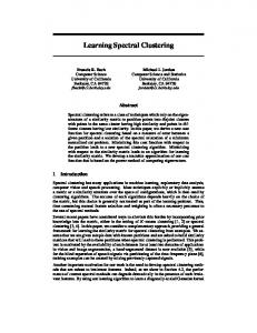
Robustness: Kernel Component Analysis original image
corrupted image
KPCA reconstruction
Weighted LS-SVM: robustness [Alzate & Suykens, IEEE-TNN 2008] ICCHA4, Hong Kong
9
Robustness: Kernel Component Analysis original image
corrupted image
KPCA reconstruction
KCA reconstruction
Weighted LS-SVM: robustness and sparsity [Alzate & Suykens, IEEE-TNN 2008] ICCHA4, Hong Kong
9
Overview
• Introduction • Kernel PCA: primal and dual model representations •
Spectral clustering
• Kernel spectral clustering • Model selection • Sparsity • Incorporating prior knowledge
Spectral graph clustering Minimal cut: given the graph G = (V, E), find clusters A1 , A2 min
qi ∈{−1,+1}
1X wij (qi − qj )2 2 i,j
with cluster membership indicator qi (qi = 1 if i ∈ A1, qi = −1 if i ∈ A2) and W = [wij ] the weighted adjacency matrix. 5 4
1 2
6
3
cut of size 2
cut of size 1 (minimal cut)
ICCHA4, Hong Kong
10
Spectral graph clustering • Min-cut spectral clustering problem min q˜T L˜ q
q˜T q˜=1
with L = D − W the unnormalized graph Laplacian, degree matrix P D = diag(d1, ..., dN ), di = j wij , giving L˜ q = λ˜ q. Cluster member indicators: qˆi = sign(˜ qi − θ) with threshold θ. • Normalized cut L˜ q = λD q˜ [Fiedler, 1973; Shi & Malik, 2000; Ng et al. 2002; Chung, 1997; von Luxburg, 2007]
• Discrete version to continuous problem (Laplace operator) [Belkin & Niyogi, 2003; von Luxburg et al., 2008; Smale & Zhou, 2007]
ICCHA4, Hong Kong
11
Spectral clustering + K-means
ICCHA4, Hong Kong
12
Overview
• Introduction • Kernel PCA: primal and dual model representations • Spectral clustering •
Kernel spectral clustering
• Model selection • Sparsity • Incorporating prior knowledge
Kernel spectral clustering: case of two clusters • Underlying model (primal representation): eˆ∗ = wT ϕ(x∗) + b with qˆ∗ = sign[ˆ e∗] the estimated cluster indicator at any x∗ ∈ Rd. • Primal problem: training on given data {xi }N i=1 N 1X 1 T min − w w+γ vi e2i w,b,e 2 2 i=1 subject to ei = wT ϕ(xi) + b, i = 1, ..., N
with positive weights vi (will be related to inverse degree matrix). [Alzate & Suykens, IEEE-PAMI, 2010] ICCHA4, Hong Kong
13
Lagrangian and conditions for optimality • Lagrangian: N N 1 T 1X 2 X αi(ei − wT ϕ(xi) − b) L(w, b, e; α) = − w w + γ vi ei − 2 2 i=1 i=1
• Conditions for optimality: ∂L =0 ⇒ ∂w ∂L =0 ⇒ ∂b ∂L =0 ⇒ ∂e i ∂L =0 ⇒ ∂αi
w= P
P
i αi
i αi ϕ(xi)
=0
αi = γviei, i = 1, ..., N ei = wT ϕ(xi) + b, i = 1, ..., N
• Eliminate w, b, e, write solution in α. ICCHA4, Hong Kong
14
Kernel-based model representation • Dual problem: V MV Ωα = λα with λ = 1/γ MV = IN − 1T V1 1 1N 1TN V : weighted centering matrix N
N
Ω = [Ωij ]: kernel matrix with Ωij = ϕ(xi)T ϕ(xj ) = K(xi , xj ) • Dual model representation:
eˆ∗ =
N X
αiK(xi, x∗) + b
i=1
with K(xi , x∗) = ϕ(xi)T ϕ(x∗). ICCHA4, Hong Kong
15
Choice of weights vi
• Take V = D
−1
where D = diag{d1, ..., dN } and di =
PN
j=1 Ωij
• This gives the generalized eigenvalue problem: MD Ωα = λDα with MD = IN − 1T D1−11 1N 1TN D −1 N
N
This is a modified version of random walks spectral clustering. • Note that sign[ei] = sign[αi] (on training data) ... but sign[e∗] applies beyond training data
ICCHA4, Hong Kong
16
Kernel spectral clustering: more clusters • Case of k clusters: additional sets of constraints min
w(l) ,e(l) ,bl
k−1
k−1
l=1
l=1
1 X (l)T (l) 1 X (l)T −1 (l) − w w + γle D e 2 2
subject to e(1) = ΦN ×nh w(1) + b11N e(2) = ΦN ×nh w(2) + b21N .. e(k−1) = ΦN ×nh w(k−1) + bk−11N (l)
(l)
where e(l) = [e1 ; ...; eN ] and ΦN ×nh = [ϕ(x1)T ; ...; ϕ(xN )T ] ∈ RN ×nh . • Dual problem: MD Ωα(l) = λDα(l), l = 1, ..., k − 1. [Alzate & Suykens, IEEE-PAMI, 2010]
ICCHA4, Hong Kong
17
Primal and dual model representations k clusters k − 1 sets of constraints (index l = 1, ..., k − 1)
(P ) :
(l) sign[ˆ e∗ ]
= sign[w
(l) T
ϕ(x∗) + bl]
ր M ց (l)
(D) : sign[ˆ e∗ ] = sign[
P
(l)
j αj K(x∗ , xj ) + bl ]
Note: additional sets of constraints also in multi-class and vector-valued output LS-SVMs [Suykens et al., 1999]
ICCHA4, Hong Kong
18
8
8
6
6
4
4
2
2
0
0
x(2)
x(2)
Out-of-sample extension and coding
−2
−2
−4
−4
−6
−6
−8
−8
−10 −12
−10
−8
−6
ICCHA4, Hong Kong
−4
−2
x(1)
0
2
4
6
−10 −12
−10
−8
−6
−4
−2
x(1)
0
2
4
6
19
8
8
6
6
4
4
2
2
0
0
x(2)
x(2)
Out-of-sample extension and coding
−2
−2
−4
−4
−6
−6
−8
−8
−10 −12
−10
−8
−6
ICCHA4, Hong Kong
−4
−2
x(1)
0
2
4
6
−10 −12
−10
−8
−6
−4
−2
x(1)
0
2
4
6
19
Overview
• Introduction • Kernel PCA: primal and dual model representations • Spectral clustering • Kernel spectral clustering •
Model selection
• Sparsity • Incorporating prior knowledge
Piecewise constant eigenvectors and extension • Definition. [Meila & Shi, 2001] Vector α is called piecewise constant relative to a partition (A1, ..., Ak ) iff αi = αj ∀xi, xj ∈ Ap, p = 1, ..., k. • Proposition. [Alzate & Suykens, 2010] Assume v v Nv (i) a training set D = {xi}N and validation set D = {x m }m=1 i=1 i.i.d. sampled from the same underlying distribution; (ii) a set of k clusters {A1 , ..., Ak } with k > 2; (iii) an isotropic kernel function such that K(x, z) = 0 when x and z belong to different clusters; (iv) the eigenvectors α(l) for l = 1, ..., k − 1 are piecewise constant.
Then validation set points belonging to the same cluster are collinear in the k − 1 dimensional subspace spanned by the columns of E v ∈ PN (l) (l) Nv ×(k−1) v R where Eml = em = i=1 αi K(xi , xvm) + bl. ICCHA4, Hong Kong
20
Piecewise constant eigenvectors and extension • Key aspect of the proof: one has (l) e∗
PN (l) (l) = i=1 αi K(xi , x∗ ) + b PN (l) (l) P (l) K(x , x ) + b α K(x , x ) + = cp i ∗ i ∗ i i∈A / p i∈Ap (l) P (l) K(x , x ) + b = cp i ∗ i∈Ap
• Model selection to determine kernel parameters and k: (k−1) (1) (2) ), Looking for line structures in the space (ei , ei , ..., ei evaluated on validation data (aiming for good generalization) • Choice kernel: Gaussian RBF kernel χ2-kernel for images ICCHA4, Hong Kong
21
Model selection (looking for lines): toy problem 1 25 0.4
20 0.3
15 10
0.1
5
(2) i,val
x(2)
0.2
e
0
0 −5
−0.1
−10 −0.2
−15
σ 2 = 0.5, BLF = 0.56
−0.3 −0.4 −0.4
−0.2
0
(1) 0.4 e i,val 0.2
0.6
−20 −25 −30
0.8
−20
−10
0 x(1)
10
20
30
−20
−10
0 x(1)
10
20
30
25 0.8
20 0.6
15 10
0.2
5
(2) i,val
x(2)
0.4
e
0
0 −5
−0.2
−10 −0.4 −0.6 −0.8 −0.4
−15
σ 2 = 0.16, BLF = 1.0 −0.2
(1) e i,val
validation set
ICCHA4, Hong Kong
0
−20
0.2
−25 −30
train + validation + test data
22
Model selection (looking for lines): toy problem 2 σ 2 = 1.20, BLF = 0.49
8
6
4
3
(2) i,val
2
x(3)
e
2
0
1 0
−1
−2
2 −2
−4
−3 2
−6 −8
0.3
−6
−4
−2 (1) e i,val
0
2
0 1
0
4
−1
x(2)
−2
−2
x(1)
σ 2 = 0.003, BLF = 1.0
0.1
3
(2) i,val
0.2
2
x(3)
0
e
−0.1
1 0
−1
−0.2
2 −2
−0.3
−0.4 −0.4
−3 2
−0.3
−0.2
(1) 0 e i,val
−0.1
validation set
ICCHA4, Hong Kong
0.1
0.2
0.3
0 1
0
−1
x(2)
−2
−2
x(1)
train + validation + test data
23
Example: image segmentation (looking for lines)
4 3
(3) i,val
2
e
1 0
−1 −2 3 2
2
1
1 0
0
−1
−1
(2) i,val
e
ICCHA4, Hong Kong
−2 −3
−2 −3
−4 −5
(1) i,val
e
24
Image ID
Image
Proposed method
Nyström method
Human
145086
42049
167062
147091
196073
62096
119082
3096
295087
37073
ICCHA4, Hong Kong
25
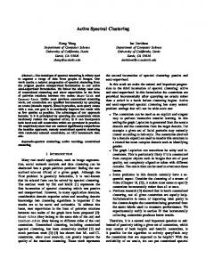
Example: power grid networks - identifying customer profiles Power load: 245 substations, hourly data (5 years), d = 43.824 Periodic AR modelling: dimensionality reduction 43.824 → 24 k-means clustering applied after dimensionality reduction
normalized load
1
0.9
normalized load
1
0.9
normalized load
1
0.9
normalized load
1
0.9
0.1
0.1
0.1
0.1
0
0
0
0.8
0.8
0.7
0.8
0.7
0.6
0.6
0.5
4
6
8
10
hour 12
14
16
18
20
22
24
0.4
0.3
0.2
2
0.5
0.4
0.3
0.2
0.6
0.5
0.4
0.3
0.7
0.6
0.5
0.4
0.8
0.7
0.3
0.2
2
4
6
8
10
hour 12
14
16
18
20
22
24
0.2
2
4
6
8
10
hour 12
14
16
18
20
22
24
0
normalized load
1
0.9
normalized load
1
0.9
normalized load
1
0.9
normalized load
1
0.9
0.1
0.1
0.1
0.1
0
0
0
0.8
0.8
0.7
0.8
0.7
0.6
0.5
0.4
0.3
0.2
2
4
6
8
10
hour 12
14
16
18
20
ICCHA4, Hong Kong
22
24
4
6
8
10
hour 12
14
16
18
20
22
24
16
18
20
22
24
2
4
6
8
10
hour
16
18
20
22
24
12
14
0.3
0.2
2
hour
0.4
0.3
0.2
10
0.5
0.4
0.3
8
0.6
0.5
0.4
6
0.7
0.6
0.5
4
0.8
0.7
0.6
2
0.2
2
4
6
8
10
hour 12
14
16
18
20
22
24
0
12
14
26
Clustering time-series: kernel spectral clustering Application of kernel spectral clustering, directly on d = 43.824 Model selection on kernel parameter and number of clusters [Alzate, Espinoza, De Moor, Suykens, 2009] 1
1
0.9
0.9
0.8
0.7
0.8
0.7
0.6
0.1
0.1
0
0
0
15
20
5
10
hour
15
20
5
10
normalized load
0.8
0.8
0.7
0.3
0.2
0.1
0.1
0
0
20
hour ICCHA4, Hong Kong
15
hour
0.4
0.3
0.2
10
0.5
0.4
0.3
5
0.6
0.5
0.4
0
0.7
0.6
0.5
20
0.8
0.7
0.6
15
normalized load
1 0.9
normalized load
1 0.9
15
0.1
hour
1
10
0.2
hour
0.9
5
0.3
0.2
0.1 10
0.4
0.3
0.2
5
0.5
0.4
0.3
0.2
0.6
0.5
0.4
0.3
0.7
0.6
0.5
0.4
0.8
0.7
0.6
0.5
normalized load
normalized load
0.8
normalized load
1 0.9
normalized load
1 0.9
0.2 0.1
5
10
15
hour
20
0
5
10
15
20
hour 27
20
1
1
0.9
0.9
0.9
0.8
0.8
0.8
0.7 0.6 0.5 0.4 0.3 0.2 0.1 0
normalized load
1
normalized load
normalized load
Clustering time-series: kernel spectral clustering
0.7 0.6 0.5 0.4 0.3 0.2 0.1
5
10
15
hour
20
0
0.7 0.6 0.5 0.4 0.3 0.2 0.1
5
10
15
hour
20
0
5
10
15
20
hour
Electricity load: 245 substations in Belgian grid (1/2 train, 1/2 validation) xi ∈ R43.824: spectral clustering on high dimensional data (5 years) 3 of 7 detected clusters: - 1: Residential profile: morning and evening peaks - 2: Business profile: peaked around noon - 3: Industrial profile: increasing morning, oscillating afternoon and evening
ICCHA4, Hong Kong
28
“Out-of-sample eigenvectors” • From the conditions for optimality: an eigenvector α satisfies α = γD −1e and 1TN α = 0. PN
• By defining deg(x) = j=1 K(x, xj ) the notion of eigenvector is extended to a validation set as follows: αval =
−1 eval [I − N1v 1Nv 1TNv ]γDval −1 evalk2 k[I − N1v 1Nv 1TNv ]γDval
satisfying kαvalk2 = 1 and 1TN αval = 0. Nv denotes the validation set size. [Alzate & Suykens, IJCNN 2011] ICCHA4, Hong Kong
29
Model selection (looking for dots): toy problem 2 badly tuned 0.03
σ = 0.003, Fisher = 1.0
0.02 0.01 3
(2) i,val
0 2
x(3)
−0.01
α
−0.02 −0.03
1 0
−1 2
−0.04
−2
−0.05
−3 2
0 (1) α i,val
−0.06 −0.05
0 1
0
0.05
−1
x(2)
−2
−2
x(1)
well tuned 0.05
σ = 1.20, Fisher = 0.12
0.04 0.03 3 2
0.01
1
x(3)
α
(2) i,val
0.02
0
0
−1 2
−0.01 −2
−0.02 −0.03 −0.04
ICCHA4, Hong Kong
−3 2
−0.03
−0.02
0 0.01 (1) α i,val
−0.01
0.02
0.03
0.04
0 1
0
−1
x(2)
−2
−2
x(1)
30
Example: image segmentation (looking for dots) 1 0.9
Fisher criterion
0.8 0.7 0.6 0.5 0.4 0.3 0.2 0.1 0 2
4
6
8
0
0.02
10
12
14
Number of clusters k
0.1
0.05
(2)
αi,val
0
−0.05
−0.1
−0.15
−0.2
−0.25 −0.04
ICCHA4, Hong Kong
−0.02
(1)0.04
αi,val
0.06
0.08
0.1
31
Overview
• Introduction • Kernel PCA: primal and dual model representations • Spectral clustering • Kernel spectral clustering • Model selection •
Sparsity
• Incorporating prior knowledge
Kernel spectral clustering: sparse kernel models original image
binary clustering
Incomplete Cholesky decomposition: kΩ − GGT k2 ≤ η with G ∈ RN ×R and R ≪ N Image (Berkeley image dataset): 321 × 481 (154, 401 pixels), 175 SV (l) e∗
ICCHA4, Hong Kong
=
P
(l)
i∈SSV αi K(xi , x∗ ) + bl 32
Kernel spectral clustering: sparse kernel models sparse kernel model
original image
Incomplete Cholesky decomposition: kΩ − GGT k2 ≤ η with G ∈ RN ×R and R ≪ N Image (Berkeley image dataset): 321 × 481 (154, 401 pixels), 175 SV (l) e∗
ICCHA4, Hong Kong
=
P
(l)
i∈SSV αi K(xi , x∗ ) + bl 32
Highly sparse kernel models on images • application on images: xi ∈ R3 (r,g,b values per pixel), i = 1, ..., N pre-processed into zi ∈ R8 (quantization to 8 colors) χ2-kernel to compare two local color histograms (5 × 5 pixels window) • N > 100.000, select subset M ≪ N based on quadratic Renyi entropy as in the fixed-size method [Suykens et al., 2002] • Highly sparse representations: # SV = 3 k • Completion of cluster indicators based on out-of-sample extensions P (l) (l) sign[ˆ e∗ ] = sign[ j∈SSV αj K(x∗ , xj ) + bl] applied to the full image [Alzate & Suykens, Neurocomputing 2011]
ICCHA4, Hong Kong
33
Highly sparse kernel models: toy example 1
4
8
3
6
2 4
1
ei
(2)
x(2)
2
0
0
−1 −2
−2
−4
−3
−6 −5
0
5
10
−4 −3
−2
−1
0
1
2
3
(1) ei
x(1)
only 3k = 9 support vectors
ICCHA4, Hong Kong
34
Highly sparse kernel models: toy example 2
4
3
2
x(2)
1
0
−1
−2
−3
−4 −4
ICCHA4, Hong Kong
−3
−2
−1
0
x(1)
1
2
3
4
35
Highly sparse kernel models: toy example 2 5 4 3 2
x(2)
1 0 −1 −2 −3 −4 −5 −5
−4
−3
−2
−1
0 x(1)
1
2
3
4
5
only 3k = 12 support vectors ICCHA4, Hong Kong
35
Highly sparse kernel models: toy example 2
4
eˆi
(3)
2
0
−2
−4 4
6 4
2 2
0 0 −2
(2) eˆi
ICCHA4, Hong Kong
−2 −4
−4
(1)
eˆi
35
Highly sparse kernel models: image segmentation *
** *
*
* * ***
* * *
* *
*
*
*
*
* *
*
* ** *
* *
* * * * ** * ** * * * * * * * * ** * * * * * * ** * * * ** ** * *** * * * * * * * * * * ** * * * * * * * * * **** * * **** * * * * ** * * * ** ** * * * * * **** * * * * * * * * * * ** * * * * ** * * * *** * * * * * * * * * *** ** * * * * * * * * * * ** * * * * * * * * * * ***** * * * * **** * ** * * * * * * * ** * * * * * ** ** ** * * *** * * * * * *** * * ** * * * ** * * * * *** * * * ** ** * * * ** * * * * ** * * *** * * ** * ** * * ** *** * * * * * ** * * * * * * * * * ** * * * ** * * *** * * * *** * * * * ** * ** * * ** * * * * * * * * * ** * * * * * * ** * ** ** * * * * ** * * ** **** * * ** * ** * * * ** * * * * * ** * *** * * * * * * ** **** ** ** * * * ** * * * * * * ** * *** * * ** * * * * * ** * * * ** * * * * * * *** * * * ** ** * * * * * ** ** * * ** * * * * * * * * ** * * * ** * * ** * * * * * ** ** * * * * * * * * ** * * * * * * * ** * * * * * * * ** * ** * * * * * * ** ** * * * * * * * * * * * * *
*
**
*
* *
*
0.5 0 −0.5
(3)
* *
* * *
* * * ** *
−1
ei
* * ** **
−1.5 −2 −2.5 −3 2 1
0.5 0
0 −1
(2)
ei
ICCHA4, Hong Kong
−0.5 −2
−1 −3
−1.5
(1)
ei
36
Highly sparse kernel models: image segmentation * * *
*
*
*
0
** *
−0.5
*
(3)
*
0.5
−1
ei
*
−1.5 −2 −2.5 −3 2 1
0.5 0
0 −1
(2)
ei
−0.5 −2
−1 −3
−1.5
(1)
ei
only 3k = 12 support vectors ICCHA4, Hong Kong
36
Overview
• Introduction • Kernel PCA: primal and dual model representations • Spectral clustering • Kernel spectral clustering • Model selection • Sparsity •
Incorporating prior knowledge
Kernel spectral clustering: adding prior knowledge • Pair of points x†, x‡: c = 1 must-link, c = −1 cannot-link • Primal problem [Alzate & Suykens, IJCNN 2009] k−1
min
w(l) ,e(l) ,bl
k−1
1 X (l)T (l) 1 X (l)T −1 (l) − w w + γle D e 2 2 (1)
l=1
l=1
(1)
subject to e = ΦN ×nh w + b11N .. e(k−1) = ΦN ×nh w(k−1) + bk−11N T
T
w(1) ϕ(x†) = cw(1) ϕ(x‡) .. T T w(k−1) ϕ(x†) = cw(k−1) ϕ(x‡) • Dual problem: yields rank-one downdate of the kernel matrix ICCHA4, Hong Kong
37
Kernel spectral clustering: example
original image
ICCHA4, Hong Kong
without constraints
38
Kernel spectral clustering: example
original image
ICCHA4, Hong Kong
with constraints
39
Conclusions • Spectral clustering within a kernel-based learning framework • Training problem: characterization in terms of primal and dual problem • Out-of-sample extensions: primal and dual model representations • Extend desirable piecewise constant property to validation level • New model selection criteria (learning and generalization aspects) • (highly) sparse kernel models • Suitable for adding prior knowledge through constraints
ICCHA4, Hong Kong
40
References Downloadable from www.esat.kuleuven.be/sista/lssvmlab/ Alzate C., Suykens J.A.K., “Multiway Spectral Clustering with Out-of-Sample Extensions through Weighted Kernel PCA”, IEEE Transactions on Pattern Analysis and Machine Intelligence, 32(2), 335-347, 2010 Alzate C., Suykens J.A.K., “Sparse Kernel Spectral Clustering Models for Large-Scale Data Analysis”, Neurocomputing, 74(9), 1382-1390, 2011 Alzate C., Suykens J.A.K., “A Regularized Formulation for Spectral Clustering with Pairwise Constraints”, International Joint Conference on Neural Networks (IJCNN 2009), Atlanta US, 2009, 141-148 Alzate C., Suykens J.A.K., “Out-of-Sample Eigenvectors in Kernel Spectral Clustering”, to appear International Joint Conference on Neural Networks (IJCNN 2011) Suykens J.A.K., “Data Visualization and Dimensionality Reduction using Kernel Maps with a Reference Point”, IEEE Transactions on Neural Networks, 19(9), 1501-1517, 2008 Suykens J.A.K., Alzate C., Pelckmans K., “Primal and dual model representations in kernel-based learning”, Statistics Surveys, 4, 148-183, 2010
ICCHA4, Hong Kong
41