Dec 5, 2012 - kernel matrix as a noisy approximation of a PSD matrix, and define a single ... 2. www-stat-class.stanford.edu/â¼tibs/ElemStatLearn/data.html .... converting the images to HSV color space and computing. SIFT features ...
1
Kernels on Sample Sets via Nonparametric Divergence Estimates
arXiv:1202.0302v2 [cs.LG] 5 Dec 2012
´ Poczos, ´ Dougal J. Sutherland, Liang Xiong, Student Member, IEEE, Barnabas and Jeff Schneider Abstract—Most machine learning algorithms, such as classification or regression, treat the individual data point as the object of interest. Here we consider extending machine learning algorithms to operate on groups of data points. We suggest treating a group of data points as an i.i.d. sample set from an underlying feature distribution for that group. Our approach employs kernel machines with a kernel on i.i.d. sample sets of vectors. We define certain kernel functions on pairs of distributions, and then use a nonparametric estimator to consistently estimate those functions based on sample sets. The projection of the estimated Gram matrix to the cone of symmetric positive semi-definite matrices enables us to use kernel machines for classification, regression, anomaly detection, and lowdimensional embedding in the space of distributions. We present several numerical experiments both on real and simulated datasets to demonstrate the advantages of our new approach.
F
1
I NTRODUCTION
Functional data analysis is a new and emerging field of statistics and machine learning. It extends the classical multivariate methods to the case when the data points are functions [1]. In many areas, including meteorology, economics, and bioinformatics [2], it is more natural to assume that the data consist of functions rather than finite-dimensional vectors. This setting is especially natural when we study time series and we wish to predict the evolution of a quantity using some other quantities measured along time [3]. Although this problem is important in many applications, the field is quite new and immature; we know very little about efficient algorithms. Here we consider a version of the problem where the input functions are probability densities, which we cannot observe directly. Instead, we have finite i.i.d. samples from them. If we can do machine learning in this scenario, then we have a way to do machine learning on groups of data points: we treat each data point in the group as a sample point from the underlying feature distribution of the group. We can then use this approach to generalize kernel machines from finite-dimensional vector spaces to the domain of sample sets, where each set represents a distribution. This problem of machine learning on groups of data points is important because in many applications, the data have natural representations as sets of data, and methods for combining these sets into a single vector for use in traditional machine learning techniques can be problematic. If we wish to find unusual galactic clusters in a large-scale sky survey or recognize certain patterns in a turbulent vector field, finding appropriate representations of these groups as feature vectors is a difficult problem in itself. Similarly, images have often • The authors are with the School of Computer Science, Carnegie Mellon University, Pittsburgh, PA, 15213.
successfully been represented as a collection of local patches, but methods for collapsing those collections into a single feature vector present problems. We therefore develop methods for classification and regression of sample sets. In the classification problem our goal is to find a map from the space of sample sets to the space of discrete objects, while in the regression problem (with scalar response) the goal is to find a map to the space of real numbers. We choose to do so by taking advantage of the support vector machine (SVM) approach; if we can define an appropriate kernel on sample sets, algorithms for classification and scalarresponse regression immediately follow. We also show how kernel machines on the space of distributions can be used to find anomalous distributions. The standard anomaly/novelty detection approach only focuses on finding individual points [4]. It might happen, however, that each measurement in a sample set looks normal, but the joint distribution of these values is different from those of other groups. Our goal is to detect these anomalous sample sets/distributions. Finally, we develop an algorithm for distribution regression. Here we handle a regression problem that has a distribution response: we find a linear map from the space of distributions to the space of distributions. As an application, we show how to use this method to generalize locally linear embedding (LLE, [5]) to distributions. To generalize kernel machines to the space of distributions, we will introduce and estimate certain kernel functions of distributions.1 The estimators are nonparametric, consistent under certain conditions, and avoid consistent density estimation. Implementations of our methods and the experiments of Section 5 are publicly available at autonlab.org. 1. By kernels we mean the kernel functions of a reproducing kernel Hilbert space. We do not use kernel density estimation in this paper.
2
2
R ELATED W ORK
We will use a generalized version of the R´enyi diver´ gence estimator of Poczos and Schneider [6]. This generalization will enable us to estimate linear, polynomial, and Gaussian kernels between distributions. There are other existing methods for divergence estimation, as well as other kinds of kernels between distributions and sets. Below we review the most popular methods, discuss some of their drawbacks, and explain why a new approach is needed. Parametric kernels: Jebara et al. [7] introduced probability product kernels on distributions. Here a parametric family (e.g. exponential family) is fitted to the densities, and these parameters are used to estimate inner products between distributions. Moreno et al. [8] similarly use Gaussian-based models to estimate Kullback-Liebler (KL) divergences in a kernel. The Fisher kernel [9] also works on parametric families only. In practice, however, it is rare to know that the true densities belong to these parametric families. When this assumption does not hold, these methods introduce some unavoidable bias in estimating inner products between the densities. In contrast, the estimator we study is completely nonparametric and provides provably consistent kernel estimations for certain kernels. Furthermore, we avoid consistent estimation of the densities, which are nuisance parameters in our problem. Nonparametric divergence estimation: Nguyen et al. [10] proposed a method for f -divergence estimation using its “variational characterization properties.” This approach involves an intractable optimization over a function space of infinite dimension. When this function space is chosen to be a reproducing kernel Hilbert space (RKHS, [11]), this optimization problem reduces to an m-dimensional convex problem, where m is the sample size. This can be very demanding in practice for even just a few thousand sample points. Sriperumbudur [12] also studies estimators that use convex or linear programming. Our approach, which uses only k-NN distances in the sample sets, can be calculated more quickly and more simply without needing to choose an appropriate kernel function for the RKHS. Sricharan et al. [13] have developed k-nearestneighbor based methods similar to our method for estimating general nonlinear functionals of a density. In contrast to our approach, however, their method requires k to increase with the sample size m and diverge to infinity. kth nearest-neighbor computations for large k can be very computationally demanding. In our approach we fix k to a small number (typically 5), and are still able to prove that the estimator is consistent. RKHS-based set kernels: There are RKHS -based approaches for defining kernels on general unordered sets as well. Kondor and Jebara [14] introduced Bhattacharyya’s measure of affinity between finitedimensional Gaussians in a Hilbert space. The method proposed by Smola et al. [15] is based on the mean
evaluations of an embedding kernel between elements of the two sets, and hence its computation time is O(m2 ). Muandet et al. [16] generalize this method to operate either on distributions or on sample sets, and provide bounds on its risk deviation. Christmann and Steinwart [17] previously showed that a similar kernel on distributions is universal and therefore SVMs based on it have good convergence properties. A closely related method which uses pairwise Euclidean distances was proposed by Szekely and Rizzo [18]. Choosing an appropriate kernel function for the RKHS can be a difficult model selection problem, however, and these methods also cannot take advantage of k-d trees and related methods to speed up computation as can ours. Our empirical evaluation will also show improved results over these methods. Quantized set kernels: Set kernels have been studied in computer vision domains as well. Image classification problems often represent images as collections of local features (c.f. Section 5.2). Perhaps the most common method for using these sets of features is to quantize the local descriptors and represent images as histograms of those features [19], the “bag of words” (BOW) method. Lyu [20] constructed composite kernels from simpler kernels defined on local features. In the pyramid matching kernel [21], each feature set is mapped to a multi-resolution histogram. These histogram pyramids are compared using a “weighted histogram intersection computation.” High-dimensional histograms can become very inefficient due to the curse of dimensionality, and selecting appropriate bin sizes is also a difficult problem. Nearest-neighbor set kernels: Boiman et al. [22] perform image classification by considering nearestneighbor distances among local descriptors (like those used in Section 5.2). They argue that in the limit, their method minimizes the KL divergence from a query image to the distribution of descriptors in the class, the optimal approach under a (dubious) Naive Bayes assumption. Tuytelaars et al. [23] kernelize this approach and integrate it with standard bag-of-features approaches, resulting in significant performance improvements. Our method uses traditional object-to-object comparisons rather than object-to-class, though in principle nothing prevents us from following the approach of [23] in defining an object-to-class kernel, and possibly combining it with the object-to-object method described here. Functional data analysis: Although the field of functional data analysis is improving quickly, there is still only very limited work available on this field. The traditional approach in functional regression represents the functions by an expansion in some basis, e.g. Bspline or Fourier basis, and the main emphasis is on the inference of the coefficients [1]. A more recent approach uses inference in an RKHS. For scalar responses, the first steps were made by Preda [24]. Inspired by this, Lian [25] and Kadri et al. [3] generalized the functional
3
regression problem to functional responses as well. To predict infinite-dimensional function-valued responses from functional attributes, they extended the concept of vector-valued kernels in multi-task learning [26] to operator-valued kernels. Although these methods have been developed for functional regression, they can be used for classifications of functions as well [27]. We note that our studied problem is more difficult in the sense that we cannot even observe directly the inputs (densities of the distributions); only a few i.i.d. sample points are available to us. Luckily, in several kernel functions we do not need to know these densities; their inner product is sufficient. Previous work: Our previous work [28] used a slightly less general form of the divergence estimator here for certain machine learning problems on distributions. Our generalized method studied below can consistently estimate many divergences, including R´enyi, KL, L2 , and Hellinger distances, in a nonparametric way. The estimator is easy to compute and does not require solving difficult kernel selection problems. That work, however, did not investigate inner product estimation or the relation to kernel machines, instead studying only simple k-NN classifiers that apply divergence estimators. The theoretical connection between several Hilbertian metrics and kernels has been studied by Hein and Bousquet [29], but they did not investigate the kernel estimation problem. Instead, we will directly define inner products on distributions based on their divergences and show how to consistently estimate them. This paper extends the results of [30], which considered classification of images, and also shows how to perform anomaly detection, regression, and low-dimensional embedding based on the same techniques.
3
F ORMAL P ROBLEM S ETTING
Here we formally define our problems and show how kernel methods can be generalized to distributions and sample sets. We investigate both supervised and unsupervised problems. We assume we have T inputs X1 , . . . , XT , where the tth input Xt = {Xt,1 , . . . , Xt,mt } consists of mt i.i.d. samples from density pt . That is, Xt is a set of sample points with Xt,j ∼ pt for j = 1, . . . , mt . Let X denote the set of these sample sets, so that Xt ∈ X . 3.1
Distribution classification
In this supervised learning problem we have inputoutput pairs (Xt , yt ) where the output domain is dis. crete, i.e. Yt ∈ Y = {Y1 , . . . , Yr }. We seek a function f : X → Y such that for a new input and output pair (X, y) ∈ X × Y we ideally have f (X) = y. We will perform this classification with support vector machines, as reviewed here. For simplicity, we discuss only the case when Y = {1, −1}. We can perform multiclass classification in the standard ways, e.g. training either (i) r one-vs-all classifiers or (ii) r(r − 1)/2 pairwise
classifiers, and then using the outputs of all classifiers to vote for the final class prediction. In our experiments we will use the second approach. Let P denote the set of density functions, K be a Hilbert space with inner product h·, ·iK , and φ : P → K denote an operator that maps density functions to the feature space K. The dual form of the “soft margin SVM” is [31]: α ˆ = arg max α∈RT
s.t.
T X
T
αi −
i=1 T X
1X αi αj yi yj Gij , 2 i,j
αi yi = 0,
(1)
0 ≤ αi ≤ C
i=1
where C > 0 is a parameter and G ∈ RT ×T is the Gram . matrix: Gij = hφ(pi ), φ(pj )iK = K(pi , pj ). The predicted class label of a test density p is then f (p) = sign
T X
! α ˆ i yi K(pi , p) + b
i=1
where the bias term b can be obtained byPtaking the average over all points with αj > 0 of yj − i yi αi Gij . There are many tools available to solve the quadratic programming task in (1), but we still must define kernel values {K(pi , p)}i and {K(pi , pj )}i,j based on the few i.i.d. samples available to us. We turn to that task in Section 4.
3.2
Distribution anomaly detection
We can use the same ideas in a one-class SVM [32] to find anomalous distributions in an unsupervised manner. To do so, we train on a set of samples considered “normal” (usually sampled randomly from a larger dataset), and estimate a function f which is positive on a region around the training set and negative elsewhere in a problem similar to (1).
3.3 Distribution regression with scalar response (DRSR) We also sometimes wish to solve a supervised task where the output domain is continuous: a regression task on sample sets with scalar response. For example, we may wish to approximate real-valued functionals of distributions such as entropy or mutual information, based on training points obtained by a reliable but computationally intensive Monte Carlo method. Alternatively, we may wish to consider images as distributions and obtain the number of pedestrians crossing a street or the size of a tumor. We can then use the same Gram matrix defined above in the support vector regression equations [31] to estimate an unknown function f : X → R.
4
3.4 Distribution regression with distribution response (DRDR) and locally linear embedding (LLE) We can also consider the regression problem where Y = X , that is, the outputs are also i.i.d. samples from distributions, and we are looking for a function f : X → X . Below we show how the coefficients of the linear regression can be calculated after transforming the distributions to the Hilbert space K. The regression problem is given by the following quadratic program: α ˆ = arg min kφ(p) − α∈RT
T X
= arg min K(p, p) − 2
T X
αi K(pi , p) +
i=1
T X
αi αj Gij .
c = arg min W
kφ(pi ) −
X
X
Wi,j φ(pj )k2K
(2)
Distribution Kernels
Many kernels, i.e. positive semi-definite functionals of p and q, can be constructed from the following form: Z Dα,β (pkq) = pα (x) q β (x) p(x) dx, (3) where α, β ∈ R. Some examples are linear,�polynomial, and Gaussian kernels exp − 21 µ2 (p, q)/σ 2 . Normally, µ2 (p, q) is the L2 distance between p and q. We can also try to use other “distances” here, such as the Hellinger distance, the R´enyi-α divergence, or the KL divergence (the α → 1 limit of the R´enyi-α divergence). These latter divergences are not symmetric, do not satisfy the triangle inequality, and do not lead to positive semidefinite Gram matrices. We will address this problem in Section 4.3. Table 1 shows the forms of these kernels and distances. TABLE 1 Kernels and squared distances we can construct with (3). R
Linear kernel Polynomial kernel L2 distance Hellinger distance
pq R �s c + pq R (p − q)2 R√ 1− pq
R´enyi-α divergence
log
R
pα q 1−α α−1
�2
D0,1 (c + D0,1 )s D1,0 − 2D0,1 + D−1,2 1 − D−1/2,1/2 � �2 log Dα−1,1−α α−1
j∈Ni
Wi,j = 1, and Wi,j = 0 if j ∈ / Ni .
j∈Ni
Note that the cost function in (2) can be rewritten as T X X X X Gii − 2 Wi,j Gij + Wi,j Wk,j Gjk . i=1
All of these methods require a kernel defined on sample sets. We choose to define a kernel on distributions and then estimate its value using our samples.
�
W ∈RT ×T i=1
s.t.
M ETHODS
i,j
LLE [5] performs nonlinear dimensionality reduction by computing a low-dimensional, neighborhoodpreserving embedding of high- (but finite-) dimensional data. As an application of DRDR, we show how to generalize LLE to the space of distributions and to i.i.d. sample sets. Our goal is to find a map f : X → Rd that preserves the local geometry of the distributions. To characterize this local geometry, we reconstruct each distribution from its κ neighbor distributions by DRDR. As above, let X1 , . . . , XT be our training set. The squared Euclidean distance between φ(pi ) and φ(pj ) is given by hφ(pi ) − φ(pj ), φ(pi ) − φ(pj )iK = K(pi , pi ) + K(pj , pj ) − 2K(pi , pj ). Let Ni denote the set of the κ nearest neighbors of distribution pi among {pj }j6=i . The intrinsic local geometric properties of distributions {pi }Ti=1 are characterized by the reconstruction weights {Wi,j }Ti,j=1 in the equation below: T X
4
4.1 αi φ(pi )k2K
i=1
α∈RT
points, and so can be generalized to distributions by simply replacing the finite-dimensional Euclidean metric 1/2 with hp − q, p − qiK .
j∈Ni
j∈Ni k∈Ni
ci,j }, we compute Yi = Having calculated the weights {W d f (pi ) ∈ R (the embedded distributions) as the vectors best reconstructed locally by these weights: Yb = arg min {Yi ∈Rd }T i=1
T X i=1
kYi −
X
ci,j Yj k2 W
j∈Ni
Finally, Yb = {Yb1 , . . . , YbT }, and Ybi corresponds to the ddimensional image of distribution pi . Note that many other nonlinear dimensionality reduction algorithms — including stochastic neighbor embedding [33, 34], multidimensional scaling [35], and isomap [36] — use only Euclidean distances between input
4.2
Kernel Estimation
We will estimate these kernel values on our sample sets by estimating Dα,β (pkq) terms for some α, β. Using the tools that have been applied for the estimation of R´enyi entropy [37], KL divergence [38], and R´enyi divergence [6], we show how to estimate Dα,β (pkq) in an efficient, nonparametric, and consistent way. . Let X1:n = (X1 , . . . , Xn ) be an i.i.d. sample from a . distribution with density p, and similarly let Y1:m = (Y1 , . . . , Ym ) be an i.i.d. sample from a distribution having density q. Let ρk (i) denote the Euclidean distance of the kth nearest neighbor of Xi in the sample X1:n \ {Xi }, and similarly let νk (i) denote the distance of the kth nearest neighbor of Xi in the sample Y1:m . The following estimator is provably L2 consistent if k > 2 max(|α|, |β|) + 1 and under certain conditions on the density (see the Appendix for details): b α,β = D
n X Bk,d,α,β ρ−dα (i) νk−dβ (i), n(n − 1)α mβ i=1 k
(4)
5
. Γ(k)2 ¯d denotes the where Bk,d,α,β = c¯−α−β d Γ(k−α) Γ(k−β) and c volume of a d-dimensional unit ball. 4.3 Positive Semi-definite Projection b α,β is a consistent estimator of Dα,β under appropriate D conditions, and thus plugging these estimators into the formulae in Section 4.1 gives consistent estimators for those kernels. The quality of kernel estimation therefore improves as the number of sample points increases. This does not, however, guarantee that the estimated Gram matrix is positive semi-definite (PSD). When we use R´enyi or other divergences instead of the Euclidean metric in the Gaussian kernel, the resulting functional itself may be asymmetric or indefinite. Additionally, estimation error may lead to a non-PSD result for any kernel. Therefore, we symmetrize the estimated Gram matrix with (G + GT )/2 and then project it to the nearest symmetric PSD matrix (in Frobenius norm) by discarding negative eigenvalues from its spectrum [39]. There are various other approaches in the literature to solve this problem. Many use an approach similar to ours, or shift all the eigenvalues by an amount large enough to make them all positive, or flip negative eigenvalues to be positive [40]. Moreno et al. [8] shift and scale the divergences with e−AD+B , but do not give details on how they choose A or B. Luss and d’Aspremont [41] instead view the indefinite kernel matrix as a noisy approximation of a PSD matrix, and define a single optimization problem to jointly find the “true” kernel and the support vectors. Ying et al. [42] and Chen and Ye [40] improve the training algorithm in that setting, but the latter’s empirical work found only small improvements over our “denoise” approach of discarding negative eigenvalues. It is also possible to directly use an indefinite kernel in an SVM-like learning problem. Haasdonk [43] provides a geometric interpretation as separating convex hulls in a pseudo-Euclidean space isometric to the kernel and gives some learning approaches. Ong et al. [44] associate such indefinite Gram matrices with a Reproducing Kernel Kre˘ın space, where an analog of the representer theorem holds; Loosli and Canu [45] give a reformulation of the Karush-Kuhn-Tucker conditions to provide more efficient learning for this problem. It is possible that this approach would yield better results, but these techniques remain not very well understood. The projection approach yields a transductive learning algorithm. If we have T training and N test exb ∈ amples and project the estimated Gram matrix G R(T +N )×(T +N ) onto the cone of PSD matrices, this symmetric PSD matrix defines a valid kernel on the training and test points, and thus the representer theorem holds on these points. It might not, however, be a valid kernel on other points not in the training and test sets. Note also that in classification and regression we need to solve the quadratic problem (1) in the training phase, using the Gram matrix of the training points only. It can be crucial
for this training Gram matrix to be PSD for QP solvers to find a solution of (1). In practice, however, we can also use this approach inductively by predicting based on unprojected kernel estimates. Although this approach is not supported by the representer theorem, it is computationally welldefined. The two approaches perform identically in the experiment of Section 5.1, and we also see good results with the inductive approach in Section 5.3. 4.4
Algorithm Summary
Fig. 1 gives pseudocode for classification. Input: T training and N testing feature sets Xt = {Xt,1 , . . . , Xt,mt } for t = 1, . . . , T + N ; T training class labels Yt ∈ {0, 1} for t = 1, . . . , T . for i, j ∈ {1, . . . , N + T }2 do b α,β (Xi kXj ) (4). Estimate Dα,β (pi kpj ) by D b i,j from this estimate. Calculate the kernel estimate G end for b := (G b+G b T )/2. Symmetrize the Gram matrix: G b Discard negative eigenvalues from the spectrum of G. Solve (1) and calculate α ˆ , b in the SVM. for j = T + 1, . . . , T P + N do T b i,j + b). Predict yˆj = sign( i=1 α ˆ i yi G end for Fig. 1. Algorithm summary for distribution classification.
5
N UMERICAL E XPERIMENTS
We now demonstrate the applicability of our method in several numerical experiments. As mentioned previously, the code and datasets used in this section are publicly available at autonlab.org. 5.1
USPS Classification
The USPS dataset2 [46] consists of 10 classes; each data point is a 16 × 16 grayscale image of a handwritten digit. The human classification error rate is 2.5%. The best algorithms, e.g. the Tangent Distance algorithm [47], achieve this error rate. This dataset is simple enough that raw images can be used as features for classifications, and even the Euclidean distances between images have high discriminative values. We can easily construct a considerably more difficult noisy version of this dataset, however, in which inner products and Euclidean distances become much less useful. Those measures disregard the proximity of pixels to one another. As resolutions increase, that information becomes more and more necessary. 2. www-stat-class.stanford.edu/∼tibs/ElemStatLearn/data.html
6
TABLE 2 Mean and std classification accuracies for various methods. See the text for descriptions.
We resized the images to 160 × 160 and normalized pixel intensities to sum to 1 for each image. We then treat each image as a probability distribution, where a 2d coordinate’s sampling probability is proportional to its (negated) grayscale value. We drew an i.i.d. sample of size 500 from each distribution and added Gaussian noise (zero mean, 0.1 variance) to each. Example noisy images are shown in Fig. 2.
Transductive orig
raw raw
noisy NP
Polynomial L2 Polynomial L2 R´enyi-.2 R´enyi-.5 R´enyi-.8 R´enyi-.9 R´enyi-.99 Hellinger
Inductive
93.5 ± .5 93.3 ± .6
Polynomial L2
82.1 ± .5 83.4 ± .4 92.7 ± .5 92.9 ± .5 93.7 ± .3 93.7 ± .3 95.8 ± .3 95.8 ± .3 95.9 ± .3 95.8 ± .3 96.1 ± .3 96.0 ± .2 96.0 ± .3 96.0 ± .3 96.0 ± .4 96.1 ± .4 94.9 ± .4 94.9 ± .3
Fig. 2. Noisy USPS dataset. We took 200 such samples from each class of the noisy dataset and performed 16 runs of two-fold crossvalidation, so that each 10-class SVM (i.e. 45 pairwise SVMs) had 1000 testing and 1000 training points. We tuned parameters in a grid search using 3-fold cross-validation on the training set, randomly picking among the configurations with the best performance. The margin penalty C was selected from the � set 2−9 , 2−6 , . . . , 221 ; the degree of polynomial kernels (both homogeneous and inhomogeneous) was selected from {1, 2, 3, 5, 7, 9}, while Gaussian kernels were tried � with kernel widths σ from 2−4 , 2−2 , . . . , 210 times the median of the nonzero elements of the Gram matrix. The mean accuracy for this 10-class problem was 93% for Gaussian kernels on the original images using pixel values as features, but only 83% on the noisy data. Polynomial kernels performed similarly. Using our estimates of the R´enyi-.9 divergence with k = 5 nearest neighbors, however, we obtained 96% accuracy on the noisy dataset with both transductive and inductive evaluation, approaching the human error rate. Results for other choices of αs in R´enyi divergence were indistinguishable, while Hellinger, L2 , and polynomial kernels performed slightly worse. Table 2 presents means and standard deviations of all the accuracies. “Raw” means that image pixels were used directly as features in computing inner products; “NP”, standing for “nonparametric,” means kernel values were estimated using (4). To demonstrate visually that our estimated kernel evaluations give more information about the structure of the noisy dataset than do Euclidean distances between raw images, we performed multidimensional scaling to 2d using ten instances of the digits {1, 2, 3, 4}. Fig. 3(a) shows the embedding using Euclidean distances between images and Fig. 3(b) the embedding using our estimate of the Euclidean distance between samples. We see that our method was able to preserve the class structure of the dataset. The letters form natural clusters, as opposed to the raw Euclidean distance, where the scaling
is uninformative. This helps explain why performance was so much better with the distribution-based kernels. 4
1 3 14 1 2 4 1 1 3 4 1 3 1 2 3 3 3 4 3 3 3 2 1 3 2 1 2 21 2 4 4
2 4 4 2 2 4
(a) using raw images
2 3 22 2 22 22 3 3 3 3 2 3 333 44 2 3 1 1 4 4 11111 4 4 1 4 4 1 44
(b) using distributions
Fig. 3. Multidimensional scaling using (a) Euclidean metric between the images, and (b) the estimated Euclidean distance between the distributions of the coordinates of the image pixels.
5.2
Natural Image Classification
We now turn to the use of our kernel for classification tasks in computer vision, in particular whole-image classification of objects and scenes. This section extends the ´ results of Poczos et al. [30]. One popular set of algorithms for image classification is based on the “bag of words” (BOW) representation. With BOW, each image is considered as a collection of visual words, so that an image of the coast might contain visual words describing patches of sky, sea and so on — though the words are not labeled and may not correspond to recognizable concepts. The locations of and dependencies among those visual words are ignored. The collection of unique visual words is called the visual vocabulary. Given a set of images, the visual words and vocabulary are often constructed as follows: 1) Select local patches from each image. 2) Extract a feature vector for each patch. 3) Cluster/quantize all the patch features into V categories. By doing this, each category of patches
7
would represent an area with similar extracted features, hopefully a visual concept such as “sky” or “window.” These V categories form the visual vocabulary, and each patch, represented by its category number, becomes a visual word. 4) Within each image, count the number of different visual words and construct a histogram of size V . This is the BOW representation of the image. The BOW representation is then typically used in kernels based on the chi-squared distance between histograms [48], or on Euclidean distance between histograms discounted by a square-root transformation [49], which are similar. Those transformations are probably successful in part because they approximate a model that does not make the unrealistic i.i.d. assumption for features [50]. Rather than performing the quantization steps, however, we represent each image directly as the set of extracted features from each patch (i.e. stopping at step (2) above; we refer to this as the “bag of features” representation, BOF). We can then apply our divergencebased kernels, or any other group kernel, to the images. Feature Extraction We extract dense SIFT features [51] using the techniques of Bosch et al. [52]. For each image, we compute SIFT descriptors at points on a regular grid with a step size of 20 pixels. In an attempt toward scale invariance, at each point we compute several SIFT descriptors, each of which is 128-dimensional, with a range of radii. After the feature extraction, each image is represented by a variable number of 128-dimensional feature vectors. We can also include color information in the SIFT features by converting the images to HSV color space and computing SIFT features independently in each color channel [52]. SIFT features at the same location with the same bin size are then concatenated together to produce a “color SIFT ” feature vector, with dimensionality 384. We use PCA to reduce the feature vectors’ dimensionality for computational expedience, and finally normalize each dimension to have zero mean and unit variance. We used the VLF EAT package [53] and its PHOW functionality to extract the SIFT features. Performance Evaluation We evaluated several kernels for image classification. Parameter tuning for the SVM’s margin penalty C and, when applicable, the Gaussian kernel width σ is performed as for the USPS dataset (Section 5.1). All kernel matrices are projected to be symmetric PSD before use. Nonparametric divergence kernels: These kernels are based on the proposed nonparametric R´enyi-α divergence estimators (NPR-α) and Hellinger distance estimators (NPH). In this high-dimensional setting, estimation of polynomial kernels and L2 distance is more difficult R and did not produce reliable results; the estimate of pq in particular was extremely poor. We use the k = 5th
nearest neighbors here. For NPR, we generally test the performance with α ∈ {.5, .8, .9, .99}. Note that as α → 1 the R´enyi-α divergence approximates the KL divergence, and when α = .5 it is twice the Bhattacharyya distance. Parametric kernels: These kernels assume the data follows a Gaussian distribution or a mixture of Gaussian distributions. We first fit the densities and then compute either the KL divergence between groups (G - KL, GMM - KL ) [8] or probability product kernels with α = .5 (G - PPK, GMM - PPK), which estimate the Bhattacharyya coefficients between the Gaussians [7]. We use three components in our GMMs. GMM - KL has no analytic form, so we use a Monte Carlo approximation with 500 samples. BOW kernels: We used BOW kernels as described previously, using the chi-square distance between histograms. We used k-means for quantization with a vocabulary size (number of clusters) of 1000 for color images and 500 for grayscale images. We also considered a kernel based on Euclidean distances between histograms processed by PLSA using 25 topics [54]. Note that in both cases, the features are quantized based on the original feature vectors, not the features after PCA. Pyramid matching kernel: We also test the vocabulary-guided pyramid matching kernel PMK [55], the preferred PMK variant for high-dimensional data. We used the authors’ implementation libpmk3 with their recommended parameters. Mean map kernel: We also consider the mean map kernel MMK [15], also known as the mean match kernel [20] to the computer vision community. The MMK between two groups of vectors X = {x1 , . . . , xm } andPY = {y1 , . . . , yn } is defined as kM M (X, Y) = m,n 1 i=1,j=1 k(xi , yj ). In other words, MMK is the avmn erage kernel matching score between every pair of points between the two groups. We let the pointwise� matching kernel � be the Gaussian kernel k(x, y) = 2 2 exp − kx − yk2 /σ , where the kernel width σ is tuned in the same way as other parameters. To avoid the high computational cost of MMK (O(mn) for each pair of groups), we randomly choose at most 500 points from each group to get MMK, so that the computation is affordable while the approximation error is small. In [20], it was argued that in MMK, good point-wise matches will be “swamped” when averaged with a larger number of bad matches. The author then proposed to exponentiate the point-wise kernels so that good matches (larger kernel values) will dominate the average. In our case of Gaussian kernels, the exponentiation is subsumed into the kernel width and will be selected by cross-validation. 5.2.1 Object Recognition We first evaluated these techniques on a simple subset of the ETH -80 dataset [56] to see basic properties of the performance. This dataset contains 8 categories of objects, each of which has 10 individual objects; there are 41 3. people.csail.mit.edu/jjl/libpmk
8
images of each such object from different viewing angles. We follow Grauman and Darrell [21] in evaluating on a 400-image subset of the dataset, selecting 5 images per object that capture its appearance from different angles. Sample images of two objects are shown in Fig. 4.
for context. The best α values are clearly in the vicinity of 1, i.e. near the KL divergence, though the performance seems to degrade more quickly when greater than 1 than when below. 0.9 0.85
Accuracy
0.8 0.75 0.7
Fig. 4. Images of two objects from the ETH -80 dataset. Each object has 5 different views in our subset.
0.65
BoW −1 −0.5 −0.2 0.1 0.2 0.3 0.4 0.5 0.6 0.7 0.8 0.9 0.99 1.01 1.1 1.2 1.3 1.4 1.5 2
0.6
0.92 0.9
´ Fig. 6. Classification accuracies on ETH -80 with Renyi-αs for twenty αs, as well as BOW.
Accuracy
0.88 0.86 0.84 0.82
5.2.2
Scene Classification
0.8 0.78
NPR−0.99
NPR−0.9
NPR−0.7
NPR−0.5
NPH
MMK
PMK
GMM−KL
G−PPK
G−KL
PLSA
BoW
0.76
Fig. 5. Classification accuracies on ETH -80.
Fig. 7. The 8 OT categories: coast, forest, highway, inside city, mountain, open country, street, tall building.
0.92 0.9 0.88 Accuracy
0.86 0.84 0.82 0.8
NPR−0.99
NPR−0.9
NPR−0.7
NPR−0.5
NPH
MMK
PMK
GMM−KL
G−PPK
G−KL
PLSA
0.78
BoW
We used color SIFT features for this dataset with bin size fixed at 6 pixels, as this problem does not require scale invariance. We reduced the vectors’ dimensionality to 18 with PCA, preserving 50% of the variance. Each image is therefore represented by 576 18-dimensional pairs. We tested the performance of classification into these 8 categories based on 2-fold cross-validation. The results from 10 random runs are shown in Fig. 5. We can see that our R´enyi-divergence kernels performed better than BOW, and much better than the other methods. In this test, BOW achieved impressive results when properly tuned. The improvement of NPR 0.9 (mean accuracy 89.93%, std dev 0.9%) over BOW (87.33%, std dev 1.4%) is statistically significant: a paired t-test shows a p-value of 2 × 10⁻³ . MMK performs at the same level as BOW, and also significantly worse than our methods. It is also interesting to see that GMM-based methods perform even worse than simple Gaussianbased methods. This may be because it is harder to choose the parameters of a GMM, or because divergences between GMMs could not be obtained precisely. PMK is not very accurate here, though it did evaluate quickly. Fig. 6 shows the performance of the R´enyi-α kernel for many values of α, along with the BOW performance
Fig. 8. Accuracies on the OT dataset; the horizontal line shows the best previously reported result [57]. Scene classification using BOF/BOW representations is a well-studied problem for which many methods have
9
5.2.3
Sport Event Classification
These kernels can also be used for visual event classification [61] in the same manner as for scene classification. We use the dataset from Li and Fei-Fei [61], which contains Internet images of 8 sport event categories: badminton, bocce, croquet, polo, rock climbing, rowing, sailing, and snowboarding. This dataset is considered more difficult than traditional scene classification, as it involves much more widely varying foreground activity than does e.g. the OT dataset.
Fig. 9. The 8 sports: badminton, bocce, croquet, polo, rock climbing, rowing, sailing, snowboarding.
Following Li and Fei-Fei [61], we used the first 130 images from each category. For each image, we extracted color SIFT features with radii of {6, 9, 12} and reduced their dimensionality to 57 (preserving 70% of the variance). As image sizes vary, each BOF group contains between 295 and 1542 feature vectors. To incorporate spatial information, we included the patches’ relative x and y locations in the feature vectors, and normalize each dimension as before. 0.88 0.84 0.8 Accuracy
0.76 0.72 0.68 0.64
NPR−0.99
NPR−0.9
NPR−0.7
NPR−0.5
NPH
MMK
PMK
GMM−KL
G−PPK
G−KL
PLSA
0.6
BoW
been proposed [52, 58, 59]. Here we test the performance of our nonparametric kernels against state-of-theart methods. We use the OT dataset [60], which contains 8 outdoor scene categories: coast, mountain, forest, open country, street, inside city, tall buildings, and highways. There are 2, 688 images in total, each about 256×256 pixels. Sample images are shown in Fig. 7. Our goal is to classify test images into one of the 8 categories. We used color SIFT features, and also append the relative y location of each patch (0 meaning the top of the image and 1 the bottom) onto the local feature vectors, allowing the use of some information about objects’ locations in the images in classification. (We chose not to include x coordinates, because horizontal locations of objects generally carry little information in these scene images). We used bin sizes of {6, 12, 18, 24, 30} so that more global information can be captured. A typical image therefore contains 1815 SIFT feature vectors, each of dimensionality 384; these are reduced by PCA to 53 dimensions (preserving 70% of the variance) and then y coordinates are appended. Each dimension of the feature vectors was finally normalized to have zero mean and unit variance. The accuracies of 10 random runs are shown in Fig. 8. Here results of 10-fold cross-validations are used so that we can directly compare to other published results. GMM - PPK is not shown because it is too low. NPR -0.99 achieved the best average accuracy of 92.11%, which is much better than BOW’s 90.26% (paired t-test p = 1.4 × 10⁻⁸ ). Notably, this 92.11% accuracy (std dev 0.18%) surpasses the best previous result of which we are aware, 91.57% [57]. For comparison, in 2-fold cross-validations the mean accuracies of NPR-0.99 and BOW are 90.85% and 88.21% respectively.
Fig. 10. Classification accuracy on the sport dataset, with the best previously reported result [62]. Fig. 10 shows the accuracies of 10 random 2-fold crossvalidations. Our R´enyi-.9 kernel again achieved the best accuracy, with 87.18% (std dev 0.46%). This performance is one standard deviation above the reported result for state-of-the-art methods such as those of Zhang et al. [62], which attained 86.7%. It is worth noting that these methods achieved significant performance increases by learning features, whereas we used only PCA SIFT. Compared to previous results, we can see that the performance of PPK and MMK methods decreased (we did not show GMM - PPK here because its accuracy is too low). The BOW method, though worse than R´ enyi-.9 with 82.42% (p = 6 × 10⁻⁹ ), again performs well, showing its wide applicability.
5.3
Turbulence Data
One of the challenges of doing science with modern large-scale simulations is identifying interesting phenomena in the results, finding them, and computing basic statistics about when and where they occurred. We present the results of exploratory experiments on using the proposed kernel to assist in this process, using turbulence data from the JHU Turbulence Data Cluster4 (TDC, [63]). TDC simulates fluid flow through time on a 3-dimensional grid, calculating 3-dimensional velocities and pressures of the fluid at each step. We used one time step of a contiguous 256 × 256 × 128 sub-grid. 4. turbulence.pha.jhu.edu
10
(a) Classification probabilities
(b) Anomaly scores
Fig. 11. Classification and anomaly scores along with velocities for one 54 × 48 slice of the turbulence data.
5.3.1
Classification
We first consider the task of finding one particular class of interesting phenomena in the data: stationary vortices parallel to the xy plane. Distributions are defined on the x and y components of each velocity in an 11×11 square, along with that point’s squared distance from the center. The latter feature was included due to the intuition that velocity in a vortex is related to its distance from the center of the vortex. We trained an SVM on a manually-labeled training set of 11 positives and 20 negatives, using a Gaussian kernel based on Hellinger distance. Some representative training examples are shown in Fig. 12. On this small training set, leave-one-out cross-validation scores varied significantly based on the random outcome of parameter tuning. In 1000 independent runs, Renyi-.9 kernels achieved mean accuracy 79%, Hellinger 82%, and L2 84%; each had a standard deviation of 5%.
5.3.2 Anomaly Detection As well as finding instances of known patterns, part of the process of exploring the results of a large-scale simulation is seeking out unexpected phenomena. To demonstrate anomaly detection with our methods, we trained a one-class SVM on 100 distributions from the turbulence data, with centers chosen randomly. Its evaluation on the same region as Fig. 11(a) is shown in Fig. 11(b). The two vortices are picked out, but the area with the highest score is a diamond-like velocity pattern, similar to Fig. 12(c); these may well be less common in the dataset than are vortices. We believe that the proposed classifiers and anomaly detectors serve as a proof of concept for a simulation exploration tool that would allow scientists to iteratively look for anomalous phenomena and label some of them. Classifiers could then find more instances of those phenomena and compute statistics about their occurrence, while anomaly detection would be iteratively refined to highlight only what is truly new. 5.4
Regression with Scalar Response
We now turn to the problem of distribution regression with scalar response (Section 3.3), showing examples of how it can be used for learning real-valued functionals of distributions from samples in a nonparametric way. (a) Positive
(b) Negative
(c) Negative
Fig. 12. Training examples for the vortex classifier.
0.00
true predicted
0.25
A classifier based on Hellinger kernels was then used inductively to evaluate groups along z-slices of the data, with a grid resolution of 2 × 2. One slice of the resulting probability estimates is shown in Fig. 11(a); the arrows represent the mean velocity at each classification point. The high-probability region on the left is a canonical vortex, while the slightly-lower probability region in the upper-right deviates a little from the canonical form. Note that some other areas show somewhat complex velocity patterns but mostly have low probabilities.
2
0.50
1
true predicted
0.75 4
8
12
16
(a) Skewness of Beta
20
00
1
2
3
(b) Entropy of Gaussian
Fig. 13. (a) Learned skewness of Beta(a, 3) distributions as a function of a ∈ [3, 20]. (b) Learned entropy of a 1d marginal distribution of a rotated 2d Gaussian distribution as a function of the rotation angle in [0, π].
11
(a) Rotated 2d Gaussians
(b) Euclidean image distances
(c) Kernel estimation
Fig. 14. (a) LLE of rotated 2d Gaussian distributions. (b) LLE using Euclidean distances between edge-detected images. The embedding failed to keep the local geometry of the original pictures. (c) LLE considering the edges as samples from unknown distributions. Nearby objects are successfully embedded to nearby places.
We first generated 350 i.i.d. sample sets of size 500 from Beta(a, 3) distributions, where a was randomly sampled from [3, 20], and used 300 sample sets for training and 50 for testing. Our goal was to learn the skewness of Beta(a, b) distributions, whose true value is √ 2(b − a) a + b + 1 √ s= (a + b + 2) ab but that we will approximate using the labeled sample sets. Fig. 13(a) displays the predicted values for the 50 test sample sets. In this experiment we used a R´enyi-.9 kernel, with regression parameter ε = 0.01 and C and σ tuned as in classification. The testing RMSE was 0.012. In the next experiment, we learned the entropy of Gaussian distributions. We generated a 2 × 2 covariance matrix Σ = CC T by drawing each element of C ∈ R2×2 from N (0, 1), obtaining Σ = [0.29 −0.57; −0.57 1.83]. We then generated 300 sample sets of size 500 with covariance matrices defined by rotating Σ: T 2×2 {N (0, M )}150 i=1 , with M = R(αi ) Σ R (αi ) ∈ R
where R(αi ) is a 2d rotation matrix with rotation angle αi = iπ/150. Our goal was to learn the entropy of the first marginal distribution H = 21 ln(2π e M1,1 ). Fig. 13(b) shows the learned entropies of the 50 test sample sets. We used the same settings as for the beta skewness; the testing RMSE was 0.058. 5.5
Locally Linear Embedding
Here we show results on locally linear embedding of distributions. This algorithm uses the linear DRDR method as a subroutine. We generated 2000 i.i.d. sample points from each of 63 rotated versions of a Gaussian distribution, with mean zero and covariance matrix R(αi ) Σ R(αi )T . Here Σ = [9 0; 0 1], i = 1, . . . , 63, and R(αi ) denotes the 2d rotation matrix with rotation angle αi = (i − 1)/20. We ran the LLE algorithm (Section 3.4) and embedded these distributions into 2d. The results are shown in Fig. 14(a). We can see that our method preserves the local geometry
(a) Original image
(b) Edge-detected
Fig. 15. An example view of the COIL object. of these sample sets: distributions with similar rotation angles are mapped into nearby points. We repeated this experiment on the edge-detected images of an object in the COIL dataset.5 We converted the 72 128x128 color pictures of a rotated 3D object to grayscale and performed Canny edge detection on them, as shown in Fig. 15. The number of detected edge points on these images was between 845 and 1158. Our goal is to embed these edge-detected images into a 2d space preserving proximity. This problem is easy using the original images, but challenging when only the edge-detected images are available. If we simply use the Euclidean distances between these edge-detected images, the standard LLE algorithm fails, as shown in Fig. 14(b). Considering the edge-detected images as sample points from unknown 2d distributions, however, the LLE algorithm on distributions yields a successful embedding, shown in Fig. 14(c). The embedded points preserve proximity and local geometry of the original images.
6
D ISCUSSION
AND
C ONCLUSION
We have posed the problem of performing machine learning on groups of data points as one of machine learning on distributions, where the data points are viewed as samples from an unknown underlying distribution for the group. We proposed a kernel on distributions and provided nonparametric methods for consistently estimating those kernels based on sample sets. 5. www.cs.columbia.edu/CAVE/software/softlib/coil-100
REFERENCES
We further demonstrated that our methods work well across a range of supervised and unsupervised tasks, matching or surpassing state-of-the-art performance on several well-studied image classification tasks and showing promising results in other areas.
12
[17]
[18] [19]
R EFERENCES [1] [2]
[3]
[4]
[5]
[6] [7]
[8]
[9]
[10]
[11]
[12]
[13]
[14] [15]
[16]
J. O. Ramsay and B. Silverman, Functional data analysis, 2nd. Springer, New York, 2005. H. Muller, J. Chiou, and X. Leng, “Inferring gene expression dynamics via functional regression analysis,” BMC Bioinformatics, vol. 9, no. 60, 2008. H. Kadri, E. Duflos, P. Preux, S. Canu, and M. Davy, “Nonlinear functional regression: a functional RKHS approach,” JMLR, pp. 374–380, 2010. V. Chandola, A. Banerjee, and V. Kumar, “Anomaly detection: a survey,” ACM Computing Surveys, vol. 41, no. 3, 2009. S. Roweis and L. Saul, “Nonlinear dimensionality reduction by locally linear embedding,” Science, vol. 290, no. 5500, pp. 2323–2326, 2000. ´ B. Poczos and J. Schneider, “On the estimation of α-divergences,” in AI and Statistics, 2011. T. Jebara, R. Kondor, A. Howard, K. Bennett, and N. Cesa-bianchi, “Probability product kernels,” JMLR, vol. 5, pp. 819–844, 2004. P. J. Moreno, P. P. Ho, and N. Vasconcelos, “A Kullback-Leibler divergence based kernel for SVM classification in multimedia applications,” in NIPS, 2004. T. Jaakkola and D. Haussler, “Exploiting generative models in discriminative classifiers,” in NIPS, MIT Press, 1998, pp. 487–493. X. Nguyen, M. Wainwright, and M. Jordan, “Estimating divergence functionals and the likelihood ratio by convex risk minimization,” IEEE Trans. Inf. Theory, vol. 56, no. 11, 2010. A. Berlinet and C. Thomas, Reproducing kernel Hilbert spaces in Probability and Statistics. Kluwer Academic Publishers, 2004. B. Sriperumbudur, “Reproducing kernel space embeddings and metrics on probability measures,” PhD thesis, UC San Diego, 2010. K. Sricharan, R. Raich, and A. Hero, Empirical estimation of entropy functionals with confidence, Tech Report, http://arxiv.org/abs/1012.4188, 2010. R. Kondor and T. Jebara, “A kernel between sets of vectors,” in ICML, 2003. ¨ A. Smola, A. Gretton, L. Song, and B. Scholkopf, “A Hilbert space embedding for distributions,” in ALT, 2007. ¨ K. Muandet, B. Scholkopf, K. Fukumizu, and F. Dinuzzo, “Learning from distributions via support measure machines,” arXiv.org, vol. stat.ML, Feb. 2012.
[20] [21]
[22]
[23]
[24]
[25]
[26]
[27]
[28]
[29]
[30]
[31]
[32]
[33] [34]
A. Christmann and I. Steinwart, “Universal kernels on non-standard input spaces,” in NIPS, 2010, pp. 406–414. G. Szekely and M. Rizzo, Testing for equal distributions in high dimension, InterStat, 2004. T. Leung and J. Malik, “Representing and recognizing the visual appearance of materials using threedimensional textons,” IJCV, vol. 43, pp. 29–44, 2001. S. Lyu, “Mercer kernels for object recognition with local features,” in CVPR, 2005, pp. 223–229. K. Grauman and T. Darrell, “The pyramid match kernel: efficient learning with sets of features,” JMLR, vol. 8, pp. 725–760, 2007. O. Boiman, E. Shechtman, and M. Irani, “In defense of nearest-neighbor based image classification,” in CVPR, IEEE, 2008. T. Tuytelaars, M. Fritz, K. Saenko, and T. Darrell, “The NBNN kernel,” in ICCV, IEEE, 2011, pp. 1824–1831. C. Preda, “Regression models for functional data by reproducing kernel Hilbert spaces methods,” J. of Statistical Planning and Inference, vol. 137, no. 3, pp. 829 –840, 2007. H. Lian, “Nonlinear functional models for functional responses in reproducing kernel Hilbert spaces,” The Canadian Journal of Stat., vol. 35, no. 4, pp. 597–606, 2007. C. Micchelli and M. Pontil, “On learning vectorvalued functions,” Neural Comput., vol. 17, pp. 177– 204, 1 2005. H. Kadri, A. Rabaoui, P. Preux, E. Duflos, and A. Rakotomamonjy, “Functional regularized least squares classication with operator-valued kernels,” in ICML, New York, NY, USA: ACM, 2011, pp. 993– 1000. ´ B. Poczos, L. Xiong, and J. Schneider, “Nonparametric divergence estimation with applications to machine learning on distributions,” in UAI, 2011. M. Hein and O. Bousquet, “Hilbertian metrics and positive definite kernels on probability measures,” in AISTATS, 2005, pp. 136–143. ´ B. Poczos, L. Xiong, D. J. Sutherland, and J. Schneider, “Nonparametric kernel estimators for image classification,” in Computer Vision and Pattern Recognition, 2012. ¨ B. Scholkopf and A. Smola, Learning with kernels: support vector machines, regularization, optimization, and beyond. The MIT Press, 2002. ¨ B. Scholkopf, J. Platt, J. Shawe-Taylor, A. Smola, and R. Williamson, “Estimating the support of a high-dimensional distribution,” Neural Computation, vol. 13, pp. 1443–1471, 7 2001. G. Hinton and S. Roweis, “Stochastic neighbor embedding,” in NIPS, MIT Press, 2002, pp. 833–840. L. Van der Maaten and G. E. Hinton, “Visualizing data using t-SNE,” Journal of Machine Learning Research, vol. 9, no. 2579-2605, p. 85, 2008.
13
[35]
[36]
[37]
[38]
[39]
[40] [41]
[42]
[43]
[44]
[45] [46]
[47]
[48]
[49]
[50]
I. Borg and P. Groenen, Modern Multidimensional Scaling: Theory and Applications. New York: Springer-Verlag, 2005. J. B. Tenenbaum, V. de Silva, and J. C. Langford, “A global geometric framework for nonlinear dimensionality reduction,” Science, vol. 290, no. 5500, pp. 2319–2323, 2000. N. Leonenko, L. Pronzato, and V. Savani, “A class of R´enyi information estimators for multidimensional densities,” Ann. of Stat., vol. 36, no. 5, pp. 2153–2182, 2008. ´ “Divergence Q. Wang, S. Kulkarni, and S. Verdu, estimation for multidimensional densities via knearest-neighbor distances,” IEEE Trans. Inf. Theory, vol. 55, no. 5, 2009. N. Higham, “Computing the nearest correlation matrix: a problem from finance,” IMA J. Num. Anal., pp. 329–343, 22 2002. J. Chen and J. Ye, “Training SVM with indefinite kernels,” in ICML ’08, 2008. R. Luss and A. d’Aspremont, “Support vector machine classification with indefinite kernels,” in NIPS, 2007. Y. Ying, C. Campbell, and M. Girolami, “Analysis of SVM with indefinite kernels,” Advances in Neural Information Processing Systems, vol. 22, pp. 2205– 2213, 2009. B. Haasdonk, “Feature space interpretation of SVMs with indefinite kernels,” Pattern Analysis and Machine Intelligence, IEEE Transactions on, vol. 27, no. 4, pp. 482–492, 2005. C. S. Ong, X. Mary, S. Canu, and A. J. Smola, “Learning with non-positive kernels,” in ICML, 2004. G. Loosli and S. Canu, “Non positive SVM,” Tech. Rep., 2010. J. Hull, “A database for handwritten text recognition research,” IEEE Trans. PAMI, pp. 550–554, 1994. P. Simard, Y. LeCun, J. Denker, and B. Victorri, “Transformation invariance in pattern recognition - tangent distance and tangent propagation,” in Neural Networks: Tricks of the Trade, ser. LNCS 1524, Springer, 1998, pp. 239–274. J. Zhang, M. Marszałek, S. Lazebnik, and C. Schmid, “Local features and kernels for classification of texture and object categories: a comprehensive study,” International Journal of Computer Vision, vol. 73, no. 2, pp. 213–238, 2006. F. Perronnin, J. S´anchez, and Y. Liu, “Large-scale image categorization with explicit data embedding,” in Computer Vision and Pattern Recognition, 2010, pp. 2297–2304. R. G. Cinbis, J. Verbeek, and C. Schmid, “Image categorization using Fisher kernels of noniid image models,” in Computer Vision and Pattern Recognition, 2012.
[51]
[52]
[53]
[54] [55] [56]
[57]
[58]
[59]
[60]
[61]
[62]
[63]
[64]
[65]
D. G. Lowe, “Distinctive image features from scaleinvariant keypoints,” International Journal of Computer Vision, vol. 60, no. 2, pp. 91 –110, 2004. A. Bosch, A. Zisserman, and X. Munoz, “Scene classification using a hybrid generative/discriminative approach,” IEEE Trans. PAMI, vol. 30, no. 4, 2008. A. Vedaldi and B. Fulkerson, VLFeat: an open and portable library of computer vision algorithms, www. vlfeat.org, 2008. T. Hofmann, “Probabilistic latent semantic analysis,” in UAI, 1999. K. Grauman and T. Darrell, “Approximate correspondences in high dimensions,” in NIPS, 2006. B. Leibe and B. Schiele, “Analyzing appearance and contour based methods for object categorization,” in CVPR, 2003. J. Qin and N. H. Yung, “Sift and color feature fusion using localized maximum-margin learning for scene classfication,” in International Conference on Machine Vision, 2010. L. Fei-Fei and P. Perona, “A bayesian heirarcical model for learning natural scene categories,” in CVPR, 2005. J. Qin and N. H. Yung, “Scene categorization via contextual visual words,” Pattern Recognition, vol. 43, 2010. A. Oliva and A. Torralba, “Modeling the shape of the scene: a holistic representation of the spatial envelope,” International Journal of Computer Vision, vol. 42, no. 3, 2001. L.-J. Li and L. Fei-Fei, “What, where and who? classifying events by scene and object recognition,” in ICCV, 2007. C. Zhang, J. Liu, Q. Tian, C. Xu, H. Lu, and S. Ma, “Image classification by non-negative sparse coding, low-rank and sparse decomposition,” in CVPR, 2011. E. Perlman, R. Burns, Y. Li, and C. Meneveau, “Data exploration of turbulence simulations using a database cluster,” in Supercomputing SC, 2007. D. Loftsgaarden and C. Quesenberry, “A nonparametric estimate of a multivariate density function,” Annals of Mathematical Statistics, vol. 36, pp. 1049– 1051, 1965. A. van der Wart, Asymptotic Statistics. Cambridge University Press, 2007.
14
A PPENDIX We give here an overview of the estimator defined in Section 4.2, which is a generalization of the work by ´ Poczos et al. [28]. k-NN Based Density Estimators k-NN density estimators operate using distances between the observations in a given sample and their kth nearest neighbors. Although we do not perform consistent density estimation, the ideas of these estimators are crucial in deriving the divergence estimator. . Let X1:n = (X1 , . . . , Xn ) be an i.i.d. sample from a . distribution with density p, and similarly let Y1:m = (Y1 , . . . , Ym ) be an i.i.d. sample from a distribution having density q. Let ρk (i) denote the Euclidean distance of the kth nearest neighbor of Xi in the sample X1:n \ {Xi }, and similarly let νk (i) denote the distance of the kth nearest neighbor of Xi in the sample Y1:m . Let c¯d denote the volume of a d-dimensional unit ball. Loftsgaarden and Quesenberry [64] define the k-NN based density estimators of p and q at Xi as pˆk (Xi ) =
k , (n − 1) c¯d ρdk (i)
qˆk (Xi ) =
k . m c¯d νkd (i)
Note that these estimators are consistent only when k(n) → ∞, as claimed in 1. We will use these density estimators in our proposed divergence estimators, but we will keep k fixed and still be able to prove their consistency. Theorem 1 (convergence in probability): If k(n) denotes the number of neighbors applied at sample size n, limn→∞ k(n) = ∞, and limn→∞ n/k(n) = ∞, then pˆk(n) (x) →p p(x) for almost all x. b α,β (X1:n kY1:m ) Consistency of D If M is the support of p, our goal is to estimate (3): Z Dα,β (pkq) = pα (x) q β (x) p(x) dx. M
Our proposed estimator (4) is equivalent to n X �−α �−β b α,β = Bk,d,α,β D (n − 1) ρdk (i) m νkd (i) , n i=1
. Γ(k)2 ¯d is the volwhere Bk,d,α,β = c¯−α−β d Γ(k−α)Γ(k−β) and c ume of a d-dimensional unit ball. d Let B(x, R) denote a closed � balld around x ∈ R with radius R, and let V B(x, R) = c¯d R be its volume. In the following theorems we will assume that almost all points of M are in its interior and that M has the following additional property: � V B(x, δ ∩ M) . � rM = inf inf > 0. 0